A Semi-Technical Primer on LLMs: Pt. 3 Modern Improvements & Extending Beyond Text

How transformer-based LLMs evolved from next-word predictors into modular, reasoning-oriented, multimodal systems.

In Part 2, we saw how LLMs turn raw transformer circuitry into a chat interface. That simple loop of predicting, appending, and repeating is powerful, but on its own it still a bit like talking to a well-read parrot. It’s often helpful, typically reliable, and even quite fast, but it can’t quite handle juggling images or plugging in to your calendar.

To graduate from a novel toy to real-world utility, LLMs leveled up on three fronts:

• Quality: Deeper reasoning, with longer memory and richer context windows

• Efficiency: Lower serving costs, sub-second latency, global-scale throughput

• Flexibility: Ability to call tools, browse fresh data, see pictures, hear speech, and even output code or images

Engineers attacked these from three angles:

1. Under the hood: Upgrading core model design, training methods, and alignment techniques to boost capabilities and make adaptation cheaper

2. At Runtime: Equipping the models with additional context, chained thought, and tools to call to improve their responses at inference

3. Beyond text: Extending the same transformer backbone to see images, hear speech, and even generate visuals or audio

In this part, we’ll unpack these upgrades and show how they collectively turned GPT‑3’s raw transformer into the foundation for GPT‑4 class systems.

Let’s get to it!

1. Upgrading the Core: Architecture, Training, & Inference

Before we give LLMs new tools or senses, we need to sharpen the core engine itself. The transformer was a breakthrough, but early models like GPT‑2 and GPT‑3 were still limited. They had short context windows, ballooning compute costs, and slow inference speeds that made them impressive demos but impractical for extensive use cases.

Researchers attacked these bottlenecks head-on, making upgrades across the three main components that go into making a model from Part 2. This section explores those three under-the-hood upgrades:

1. Core architecture improvements that expand context, efficiency, and reasoning ability.

2. Training and adaptation methods that stabilize scaling, cut fine-tuning costs, and improve alignment.

3. Inference-time efficiency gains that slash latency and serving costs.

These under-the-hood changes are why today’s LLMs feel smarter, faster, and cheaper than their predecessors.

1.1 Core Architecture Improvements

For architectural improvements, we’ll look at three key upgrades that strengthened the transformer’s core design and unlocked more capable, context-aware models without changing its fundamental blueprint:

• Positional encodings: More flexible methods for encoding token order that scale to far longer contexts and improve reasoning over relative positions.

• Attention efficiency (Multi-Query / Grouped-Query): Architectural tweaks that restructure attention heads to reduce memory bandwidth demands while preserving output quality.

• Mixture of Experts (MoE): Conditional routing layers that expand model capacity without proportional increases in compute cost.

Let’s start with positional encodings, where a subtle shift in how models track token order allowed transformers to handle vastly larger inputs and reason more effectively across them.

1.1.1 Improving Positional Encodings: RoPE

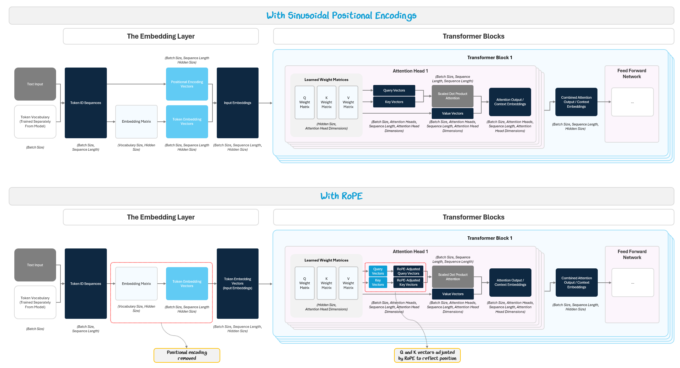
As we saw from Part 2, the model doesn’t inherently understand the order of tokens, so we added sine and cosine positional encodings to the input embeddings to help.

While these wave-like patterns effectively conveyed position, they were fixed and rigid. They assume position changes smoothly, like a sine wave, when in reality, language often has abrupt transitions (e.g., shifts between paragraphs) and nuanced positional cues that rigidly structured sine waves can’t capture.

To overcome these constraints, researchers introduced Rotary Positional Embeddings (RoPE), used in models like GPT‑4. RoPE was a key advancement because it:

• integrates position directly into the attention mechanism, allowing models to reason about relative distances between tokens instead of relying solely on absolute positions

• scales far more efficiently to longer context lengths without retraining or interpolation tricks, making it well-suited for the massive context windows used in modern LLMs.

To do this, RoPE applies position during attention by rotating the query and key vectors in high-dimensional space based on each token’s position, instead of appending a position signal to token embeddings.

Here’s the intuition:

• First, we embed the tokens as usual, but do not add a positional encoding.

• Inside attention, we “rotate” the query and key vectors slightly depending on their positions: token #1 rotates a little, token #10 rotates more, token #100 rotates even more.

• When attention is computed, it measures how aligned these rotated queries and keys are.

Because the rotation encodes relative position, attention naturally “knows” how far apart tokens are. Separate positional rules are not needed.

The below GIF shows how a query or key vector is rotated based on position (again) using sine and cosine functions. RoPE splits its dimensions into pairs: (0,1), (2,3), (4,5), etc. It then applies the 2D rotation independently to each pair, encoding positional information directly into the queries and keys, allowing attention to naturally account for both meaning and relative position.

Source

By rotating queries and keys within attention, rather than adding fixed signals to embeddings, RoPE provides a smooth, mathematically grounded way to represent position. It generalizes to longer sequences and naturally captures relative position better than older methods.

The underlying math is intricate, but the idea to remember is simple: rotate queries and keys so attention sees both meaning and position at once. If you’d like to go deeper, this video is an excellent explainer:

If you didn’t get this…
RoPE weaves position directly into attention by rotating Q and K vectors, so the model “feels” how far apart words are. It’s a cleaner, more scalable way to represent position than older fixed patterns like creating a dedicated positional encoding vector.

1.1.2 Multi-Query / Grouped-Query Attention

Standard multi-head attention creates separate key (K), value (V), and query (Q) vectors for each head. This improves quality but expensive at inference: every head stores its own KV cache, so memory usage scales linearly with the number of heads. For large models with dozens of heads and long contexts, this becomes a major bottleneck.

Grouped-Query Attention (GQA) addresses this by grouping heads together to share keys and values. Instead of every head maintaining its own KV cache, a small group of heads reuses the same K/V while still keeping separate queries. This significantly reduces KV cache size and speeds up inference, while preserving some of the diversity of standard multi-head attention.

Multi-Query Attention (MQA) takes this idea further: rather than grouping heads, it shares a single K/V cache across all heads. Each head still has its own queries (Q), but they all attend to the same K/V. This maximizes efficiency, cutting KV cache size down to “1 × context length”, but can slightly reduce modeling flexibility compared to GQA.

The tradeoff is speed versus flexibility. GQA keeps more diversity because each group of heads has its own K/V cache, which helps preserve quality. MQA is faster and lighter but forces all heads to share one K/V cache, which can reduce nuance in what the model pays attention to.

In practice, modern LLMs often use GQA as the default (e.g., GPT-4) because it balances speed and quality, while MQA is favored in scenarios where latency and memory are the top priorities.

If you didn’t get this…
Instead of every attention head keeping its own memory, GQA makes small groups share, and MQA makes all heads share one. This cuts memory and speeds things up, with GQA balancing quality and MQA maximizing efficiency. It’s like students sharing one set of lecture notes instead of everyone writing their own, trading detail for efficiency.

1.1.3 Mixture of Experts (MoE)

A key bottleneck in transformers is that every token passes through every parameter in every layer. Dense models like GPT‑3 or GPT‑4 run every neuron in their feedforward layers for every token, even if most aren’t needed. This provides a lot of power capacity but is inefficient.

Mixture of Experts (MoE) changes that by replacing certain feedforward (FFN) layers in the transformer with MoE layers. These layers contain many parallel “expert” FFNs, plus a gating network that routes each token to a small subset of experts (often the top 1–2).

Here’s how it works:

1. Shared Attention: Each block still begins with dense self-attention, where all tokens see the same context.

2. Gating: After attention, a lightweight gate (a router) looks at each token and picks the most relevant expert(s).

3. Sparse Feedforward: Only those chosen experts process the token, and their outputs are merged back.

4. Residual Connection: The token rejoins the shared stream for the next layer.

Source (Modified)

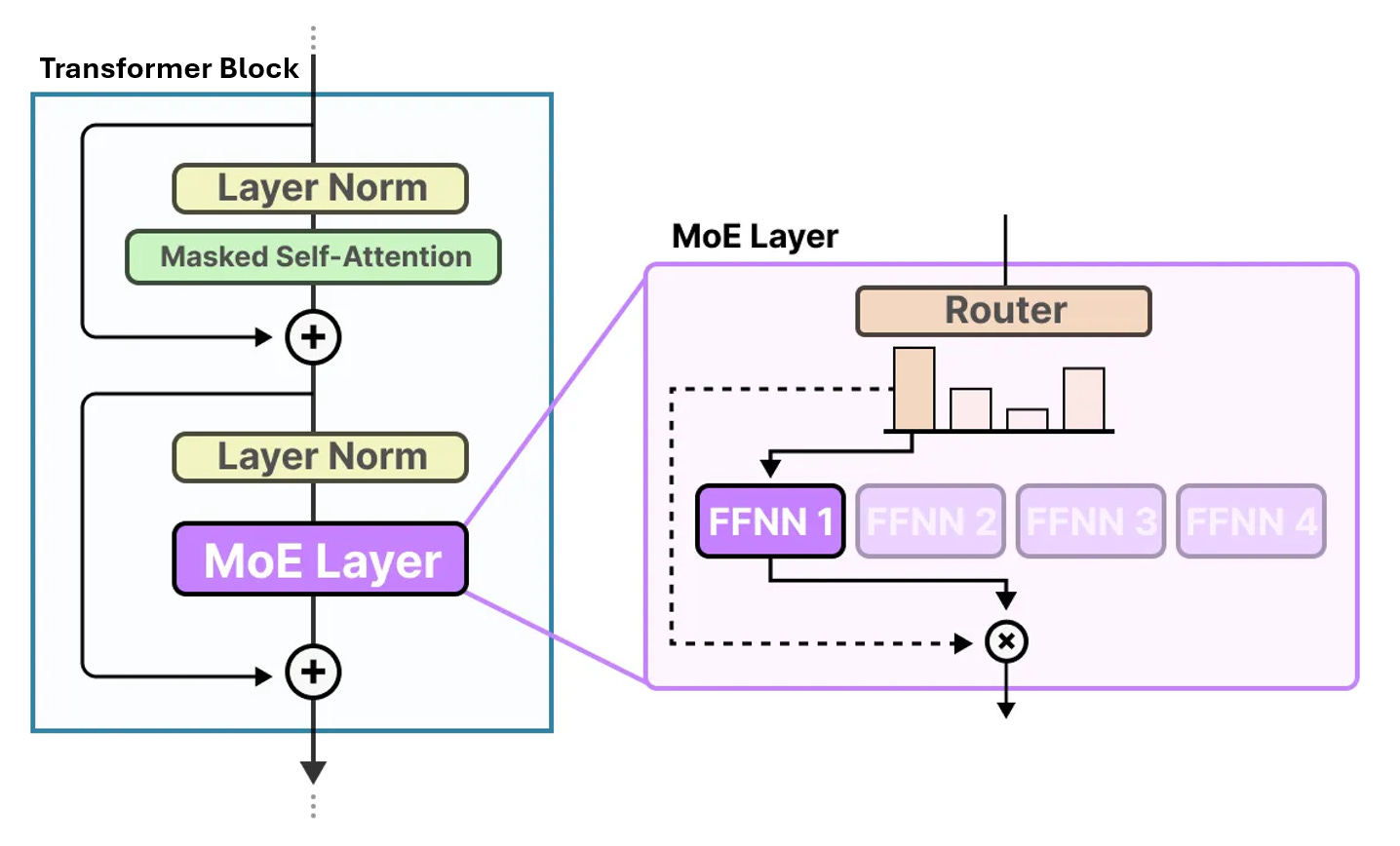
As this goes through multiple layers of transformer blocks, different experts may be called.

Source

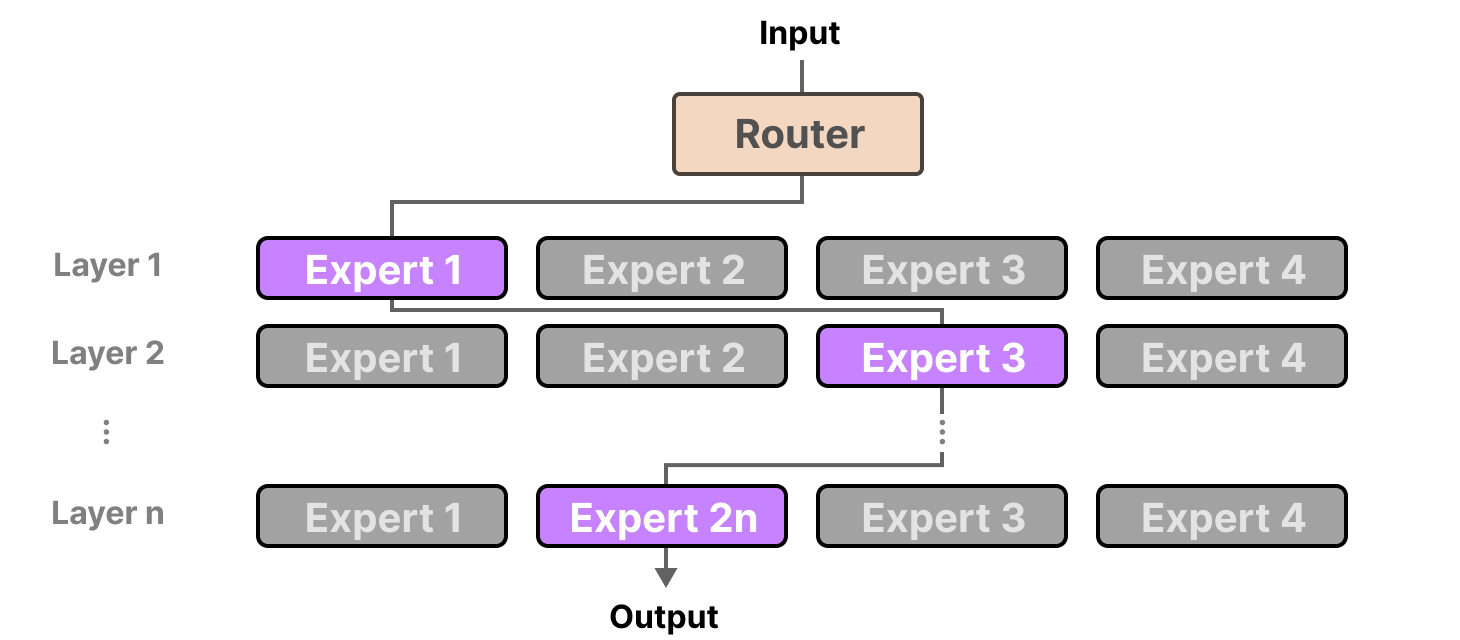
Note that experts in different layers are separate sets of parameters. This allows hierarchical specialization. Early MoE layers may capture low-level token or syntax patterns. Later MoE layers may specialize in higher-level abstractions (semantics, reasoning steps).

This structure allows a model to have hundreds of billions of parameters, but activate only a fraction per token, scaling capacity without proportional cost. This is how a trillion-parameter MoE model can run at a compute cost closer to a dense model with a fraction of those parameters.

If you didn’t get this…
MoE layers are like specialist breakout rooms after a shared meeting, everyone attends the global attention session, but then each token is routed to just the specialists it needs before regrouping.

1.2 Training & Adaptation Methods

Improving the transformer’s architecture made models more capable, but raw scale alone isn’t enough. To be useful, these systems need two things: a way to adapt cheaply to new tasks and better way to align with human preferences.

Early GPT-style models required expensive full-model fine-tuning and relied on labor-intensive human feedback loops. Modern LLMs solved these bottlenecks with two breakthroughs:

• Parameter-efficient fine-tuning (LoRA, QLoRA): Techniques that make it practical to specialize massive models without retraining billions of weights.

• Alignment methods (RLAIF, SRPO, GRPO): A progression from human-labeled feedback to scalable, AI-assisted preference optimization.

These advances further transformed base models from general-purpose text generators into more capable steerable assistants that can be rapidly adapted to new domains and aligned to user intent.

1.2.1 Parameter-Efficient Fine-Tuning: LoRA and QLoRA

Training a large language model from scratch can cost tens to hundreds of millions of dollars because of the scale. This is so much so that even full fine-tuning (i.e., updating every weight for a specific domain or task) can be prohibitively expensive.

Instead, researchers developed parameter-efficient fine-tuning (PEFT) methods: techniques that adapt massive pretrained models by updating only a tiny fraction of their weights. The base model stays frozen, and small “adapter” parameters are trained to steer its behavior. Instead of retraining the entire network, these approaches focus on small, efficient add-ons or scaling factors that tweak the model’s outputs without disturbing its core weights.

Low-Rank Adaption (LoRA) implements PEFT by inserting small, low-rank matrices alongside frozen weights and trains only these adapters, dramatically cutting the number of trainable parameters.

Imagine we have a massive, finely tuned machine (the pretrained LLM). It works well overall, but we want it to perform slightly differently to better write legal contracts instead of casual emails. Rebuilding the whole machine or re-tuning every part (full fine-tuning) would be slow, costly, and risky.

LoRA is like adding a small adapter on top of the machine instead of re-engineering it from scratch.

• The big model stays frozen and untouched (all its knowledge intact).

• LoRA adds tiny low-rank "side modules" (Wa and Wb) alongside certain layers.

• During training, only these adapters learn to “nudge” the model’s outputs in the right direction for our task.

• At inference, the base model and the adapter outputs are combined, steering the frozen model without rewriting it.

This diagram shows how LoRA fine-tunes a model without updating all its weights. On the left, we see the frozen pretrained weight matrix (W) from the base model. Inputs (x) pass through these weights to produce an embedding (h).

Source

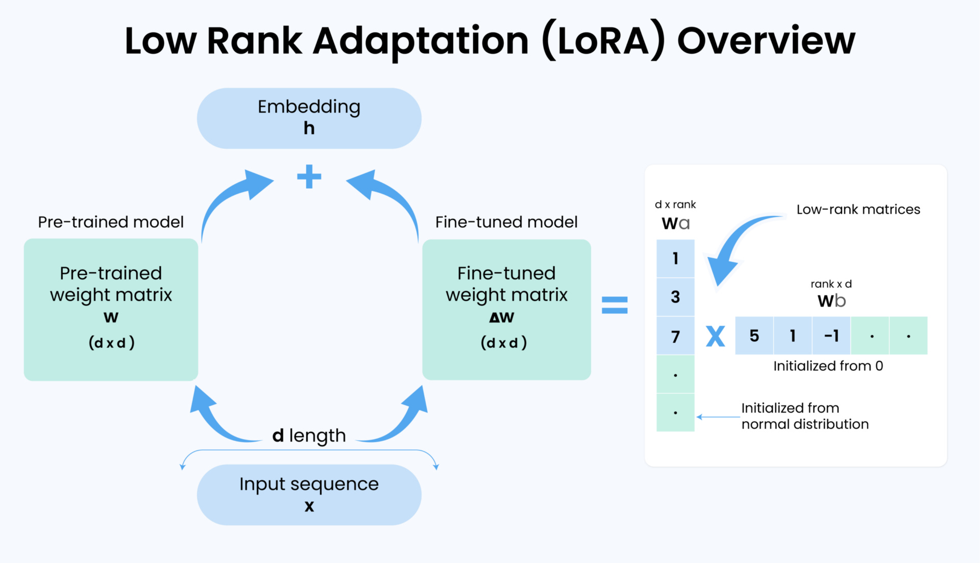
Here, h is the output of the weight matrix being adapted. In practice, LoRA is often attached to specific linear layers within the model (e.g., attention projections), so h would be the result of those projections plus the LoRA adjustment.

On the left, we see how a normal model works: the input (x) goes through the big frozen weight matrix (W) and produces an output (h). In full fine-tuning, we’d adjust every number in W to train the model. This is a huge, expensive job.

On the right, LoRA takes a shortcut. Instead of changing W, it adds a tiny side-path:

• First, Wa squeezes the input down to a small, simpler version (like distilling it into its essentials).

• Then, W_b expands it back up, creating a small "correction signal."

This correction is added on top of the frozen model’s output, gently steering it toward the new task. During training, the model’s loss is sent backward through the network via backpropagation. Because the base weights are frozen, only the small LoRA matrices (Wa​ and Wb) receive updates, learning how to add just the right correction signal to steer the frozen model toward the new task.

Because these adapters are so small, they’re cheap to train and can be swapped in or out. It’s like leaving the big engine alone but attaching a small control knob that’s easy to turn.

Source

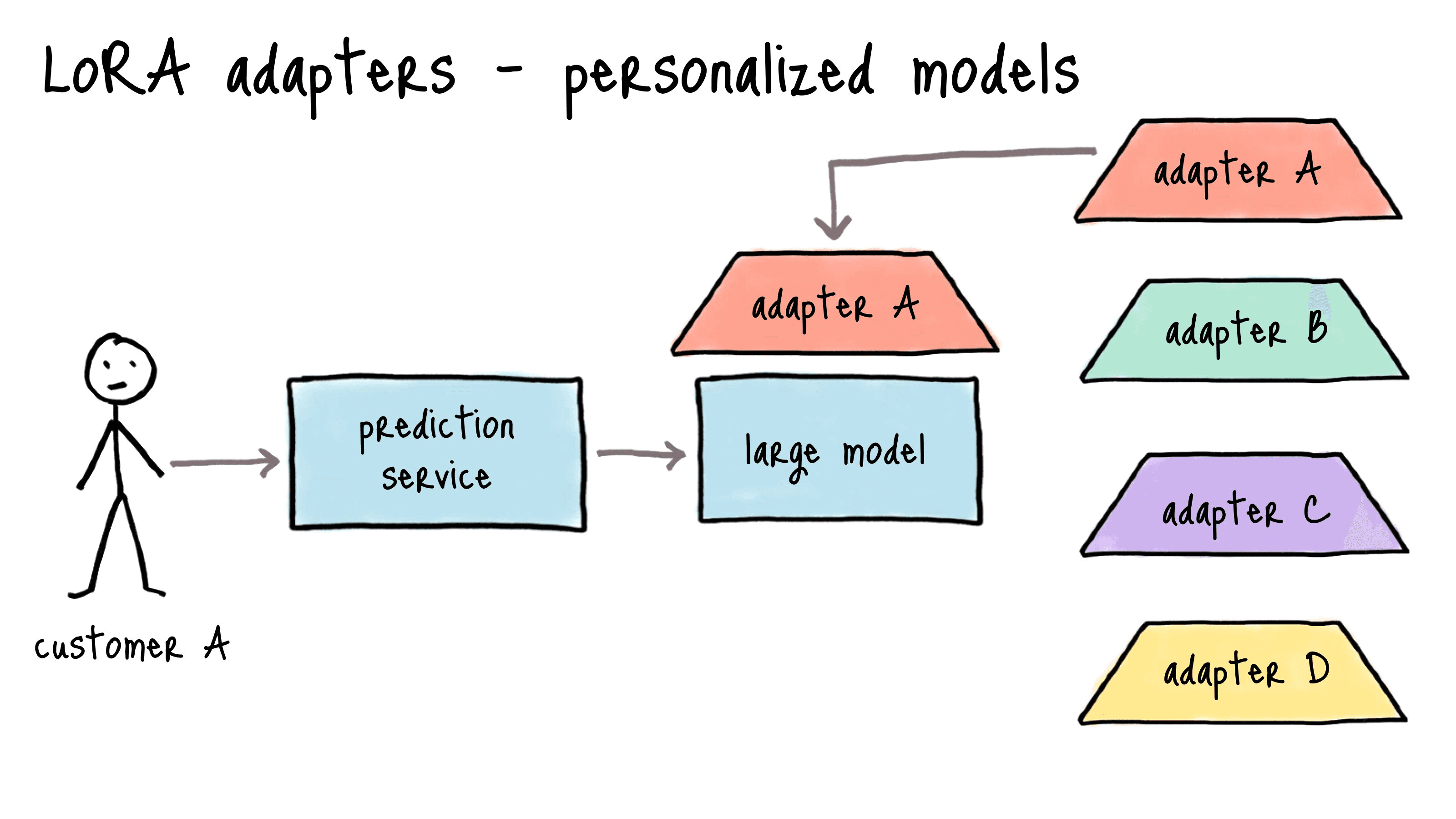
This means organizations can maintain a single, powerful base model while spinning up lightweight, task-specific adapters on demand. This unlocks personalization at scale without the cost of training or hosting separate models.

Even with LoRA’s efficiency, large models still require huge memory footprints just to store their frozen weights during fine-tuning. Quantized LoRA (QLoRA) solves this by combining LoRA with quantization.

• First, the base model’s weights are compressed from high precision (16-bit or 32-bit) down to 4-bit integers (quantized).

• The quantized weights stay frozen during training.

• On top of this compact backbone, LoRA adapters are added and trained exactly as before.

Because the adapters are tiny and the base model is stored in low precision, QLoRA makes fine-tuning massive models practical on consumer GPUs, while retaining nearly the same performance as higher-precision setups.

LoRA and QLoRA make it possible to adapt massive models using less than 1% of the compute and parameters required for full fine-tuning. Instead of retraining the entire network, we simply train small, efficient adapters on top of a frozen base model. This modularity means one foundation model can power countless specialized variants without retraining from scratch. Combined with quantization (QLoRA), even huge models can now be fine-tuned on affordable hardware.

If you didn’t get this…
PEFT, LoRA, and QLoRA are like adding a small steering knob to a giant machine. You don’t rebuild the engine, you just learn how to turn it in the right direction.

1.2.2 Enhanced Alignment Methods: RHLF, RAILF, SRPO, GRPO

In Part 2, we introduced RLHF and DPO as ways to align models with human preferences. They worked well but shared a bottleneck: human feedback doesn’t scale. RLHF required costly ranking and complex reinforcement loops, while DPO still depended on large pools of labeled preferences.

To break this bottleneck, researchers automated feedback and simplified training. RLAIF uses aligned teacher models (often guided by explicit constitutions) to generate preference data at scale. SRPO and GRPO extend DPO’s direct optimization to large, AI-ranked datasets, eliminating reinforcement learning entirely. Together, these methods replaced slow human loops with scalable synthetic pipelines, making alignment faster, cheaper, and broader.

1.2.2.1 RLAIF

The next wave of methods tackled this by automating the feedback loop. Reinforcement Learning from AI Feedback (RLAIF) replaced most human raters with an aligned “teacher” model. Instead of hiring humans to rank responses, a strong model, already aligned using earlier methods, evaluates candidate outputs and assigns preference labels. Humans still oversee the process, but their role shifts to auditing the teacher’s decisions rather than manually scoring every response.

Source

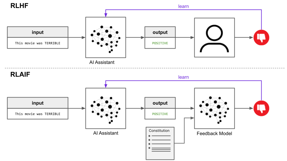
Crucially, this teacher model is often guided by a “constitution”: an explicit set of written principles about safe and ethical behavior. This “constitutional AI” setup is particularly useful for safety-critical alignment, since it allows models to be trained both helpful and harmless objectives, filtering out unsafe, biased, or undesirable outputs according to predefined rules.

If you didn’t get this…
RLAIF uses an aligned AI “teacher” to label good and bad answers, with humans just auditing. It’s faster, cheaper, and guided by clear rules (a “constitution”) to keep models safe.

1.2.2.1 SRPO

Self-Improving Robust Preference Optimization (SRPO) is an alignment method that extends DPO by introducing a self-improvement mechanism within a robust optimization framework.

Instead of using reinforcement learning or separate reward models, SRPO trains a language model together with a “revision policy” that improves its own answers step by step. In this setup, the revision policy suggests better responses, and the model learns to prefer these improved versions over its original ones. The revision policy is another policy (often initialized from the same base LM) trained to take a response y and propose a revised, better response y′. This is done iteratively. The revision policy sees the original response plus the prompt and tries to rewrite it into something preferable (more factual, more helpful, etc.).

By using existing preference data and allowing the model to refine itself through these revisions, SRPO becomes more robust to new or unusual inputs and can scale without needing extra human feedback. In tests, it has outperformed standard DPO, showing big improvements in both preference win rates and factual accuracy, making it an effective and scalable way to align models.

If you didn’t get this…
SRPO lets a model improve itself: it drafts better answers, learns to prefer them, and repeats. This scales alignment without humans or complex reinforcement training. It’s like editing your own rough drafts until they’re polished, without needing an external editor.

1.2.2.3 GRPO

Group Relative Policy Optimization (GRPO) is a simpler and more efficient way to train language models on reasoning-heavy tasks. Instead of using a separate “value model” like traditional PPO, GRPO works by having the model generate several answers to the same question, scoring them, and then comparing each answer to the group’s average. The model is then updated to favor the better answers while reducing the likelihood of weaker ones, but with limits in place to prevent it from changing too much at once.

By using this group-based approach, GRPO lowers the memory and compute needed for training while still keeping updates stable and effective. This method has been especially successful for improving reasoning skills in models like DeepSeekMath and DeepSeek-R1, helping them reach top performance on math and logic tasks much more efficiently than older training methods.

If you didn’t get this…
GRPO improves reasoning by having a model compare its own answers, learn from the best ones, and drop the worst. No extra value model or heavy reinforcement training required. It’s like brainstorming several answers, then picking and refining the best one while discarding the weaker ones.

1.2.2.4 Recapping Alignment Improvements

These methods shift alignment from human-heavy RL to AI-led direct optimization. RLAIF uses teacher models to replace most human raters, while SRPO and GRPO extend optimization with scalable AI feedback and self-improvement. Together, they make alignment faster, cheaper, and more practical for today’s largest models.

1.2.3 Other Upgrades

Alongside LoRA and alignment breakthroughs, modern LLMs also benefited from lower-level engineering advances that made large-scale training feasible. These are less visible to end users but critical for enabling trillion-parameter training runs:

• Mixed-Precision Training (BF16 / FP8): Uses lower-precision number formats to cut memory and compute costs nearly in half while preserving accuracy.

• Activation Checkpointing: Saves only a subset of activations during forward passes and recomputes the rest during backpropagation, reducing memory usage.

• Optimizer State Sharding (ZeRO): Distributes the optimizer’s stored gradient history across GPUs, reducing memory per GPU and enabling training of extremely large models.

1.3 Inference Efficiency Gains

With a more capable model now, engineers also focused on inference-time efficiency to reduce serving costs and speed up generation without changing what the model has learned.

In this section, we’ll look the following key improvements:

• Speculative Decoding: A draft-and-verify approach that accelerates token generation by combining smaller “helper” models and a larger “verifier” model.

• FlashAttention: A re-engineered GPU kernel that computes attention faster while using far less memory.

• Paged Attention: A memory manager that enables ultra-long contexts by paging key-value caches between GPU and CPU memory.

These inference-time advances are invisible to the end user but crucial: they’re the reason modern LLMs can deliver sub-second responses at scale instead of timing out under the weight of their own compute demands.

1.3.1 Speculative Decoding

Speculative decoding speeds up inference by using a smaller, faster “draft model” to propose several tokens at once and a larger model to verify them in a single pass.

Source

The larger model then checks them in parallel. If the guesses match what the large model would have generated, they’re accepted immediately; if not, generation falls back to the large model for that step.

Let’s say the input is “What’s your name?”. The large model keeps its cached key and value vectors from the input tokens (1-4) and has the small model generate tokens. Let’s say the small model outputs “My name is Bob”, tokens (5-8). The large model performs a pre-fill forward pass (like from inference in Part 2) over those tokens using the cache, computing logits for all of them in parallel.

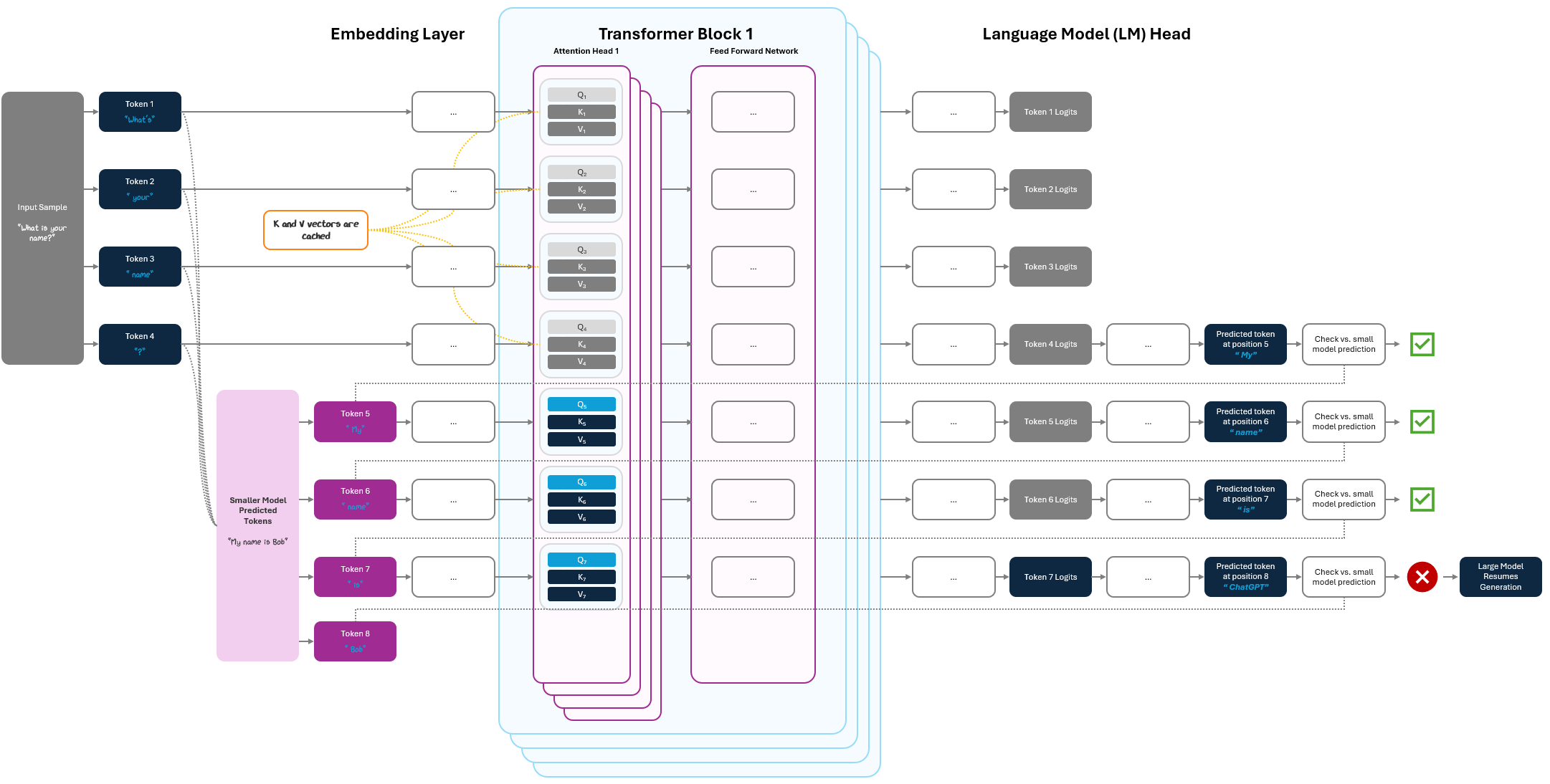
Within that single pass, it sequentially checks whether each small model prediction matches what it would have generated: if tokens match (tokens 5-7), they are accepted and the model jumps ahead. If a mismatch occurs (token 8), the large model falls back to standard autoregressive decoding from that point onward.

Because the small model is cheap to run and most of its guesses are correct, this dramatically reduces how often the big model has to run.

Look how much faster it made Google search AI!

Source

This approach cuts latency and lowers inference costs without changing output quality, since the large model still validates every token.

If you didn’t get this…
Speculative decoding is like having a faster, cheaper junior assistant rapidly draft several lines while a senior expert simply reviews and approves them, rather than writing everything from scratch.

1.3.2 Faster Attention: FlashAttention

RoPE helped models understand token order and scale to longer contexts, but attention was still painfully slow and memory-hungry. Every extra token exponentially increased the work: if we doubled our input length, memory and compute roughly quadrupled because each token has to "look at" every other token. For short prompts, that's fine but at 32k+ tokens, GPUs run out of memory fast.

FlashAttention, introduced in 2022, tackled this bottleneck by rethinking how attention is computed at the GPU level. Instead of storing huge intermediate matrices (which eat memory), it streams the calculation in smaller chunks directly through super-fast GPU registers.

The math stays the same, but the implementation changes:

• Vanilla attention: Loads all data, builds giant matrices in memory, then processes them, wasting time and GPU memory.

• FlashAttention: Breaks the process into small pieces, keeps them in fast memory (registers), and fuses steps together so nothing bulky ever touches slow memory (HBM).

The diagram compares standard attention (left) with FlashAttention (right).
In standard attention, the model loads entire matrices into memory, writes and reads them repeatedly, and only then computes attention. This eats up memory.

Source

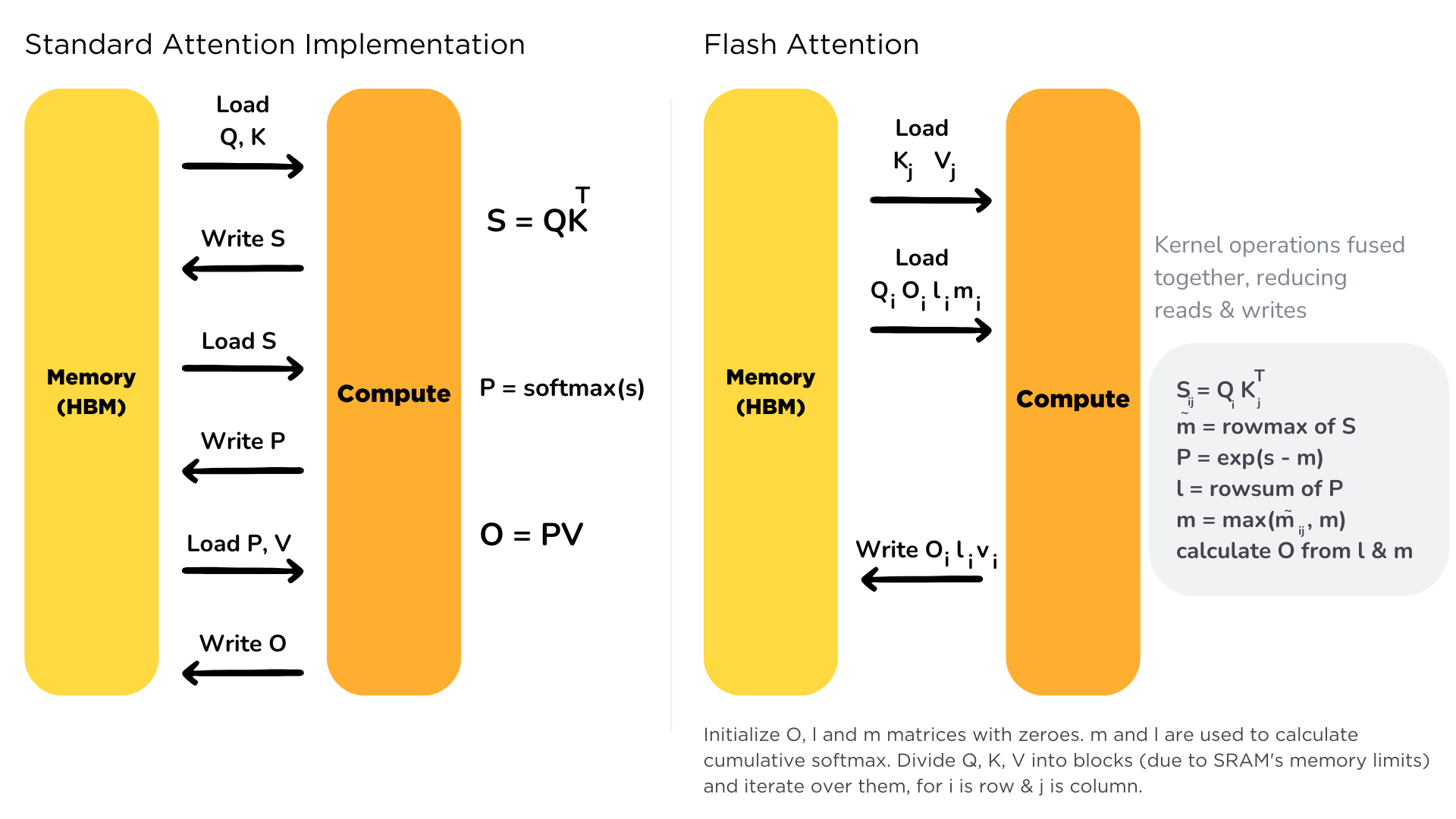
FlashAttention instead breaks the process into smaller chunks, computes them on the fly in fast GPU registers, and fuses steps together. The result: the same attention output, but with far fewer memory reads/writes and much faster performance.

This optimization massively reduces memory usage and speeds up attention, making long-context LLMs practical without changing the underlying math.

If you didn’t get this…
FlashAttention is just a smarter way to run the same math: it processes attention in small pieces using fast memory instead of creating one big, slow matrix. This makes attention dramatically faster and less memory-hungry without changing how it works.

1.3.3 Paged Attention

Even with KV caching, one of the biggest bottlenecks in LLM inference is memory usage for long contexts. As models process more tokens, they store key and value vectors in a cache so they don’t have to recompute attention over past tokens. But this cache grows linearly with context length and must stay in fast GPU memory, quickly consuming VRAM for very long prompts.

Paged Attention solves this by treating the KV cache like a virtual memory system. Instead of keeping all key-value pairs in one giant contiguous block on the GPU, it splits them into fixed-size “pages” that can be loaded and unloaded as needed, similar to how an operating system manages RAM and disk. When the model attends over past tokens, it dynamically fetches only the relevant pages into GPU memory. Pages that aren’t actively needed are offloaded to slower but larger CPU RAM and pulled back in on demand.

This makes huge contexts practical within GPU memory constraints. It’s also fully compatible with KV caching, meaning paged attention doesn’t change how the model computes attention, only how it manages memory.

If you didn’t get this…
Imagine reading a long book. You don’t keep every page spread out on your desk; you keep the pages you’re using in front of you (GPU memory) while the rest stay in the book (CPU memory) until you flip back to them. Paged Attention works the same way for tokens, letting LLMs handle massive context windows efficiently without needing absurdly large GPUs.

1.4 Recapping the Core Upgrades

At their core, these upgrades attacked the key constraints that held early GPT models back, improving their usefulness and usability:

• Attention Bottlenecks: Early transformers struggled with attention's quadratic demands since every new token meant exponential increases in memory and compute. Upgrades like RoPE, Grouped/Multi-Query Attention, and FlashAttention fundamentally unlocked longer contexts, deeper reasoning, and faster inference.

• Memory Constraints: The massive weights, enormous optimizer states, and ballooning key-value caches overwhelmed GPU memory hampered models by their sheer size. Techniques like Mixed-Precision Training, ZeRO Optimizer Sharding, and Paged Attention introduced smarter, hierarchical memory management that dramatically reduces costs and expands feasible model scale.

• Compute and Adaptation Costs: Pure scale came with prohibitive computational and adaptation expenses. Innovations directly targeted these cost barriers:

  • Mixture of Experts (MoE) introduced selective computation, routing tokens only to relevant subsets of parameters, drastically increasing model capacity without proportionally scaling compute.

  • LoRA and QLoRA shifted fine-tuning from expensive full-model retraining to lightweight, modular adapters that let organizations specialize powerful models cheaply and rapidly on consumer-grade hardware.

• Alignment and Human Feedback Efficiency: Early alignment methods relied heavily on costly human-labeled data (RLHF). Newer methods like RLAIF and SRPO harnessed AI-generated feedback and synthetic ranking, significantly reducing the bottleneck imposed by manual annotation, enabling faster, more scalable alignment processes.

A key takeaway is that most of these upgrades are less about radical architectural changes and more about engineering efficiency: smarter attention, memory, and training pipelines. These optimizations remove scaling bottlenecks so models can grow in size and quality via more depth (layers), width (hidden size), attention heads / size, and context windows.

Modern improvements (so far) have not been largely focused on reinventing transformers, we’re largely clearing the path to make bigger, better models affordable and practical so valuable AI assistants are accessible to all.

2. Runtime Intelligence: From Static Text to Grounded, Action-Taking Systems

Even with all these updates that make them powerful, LLMs still operate in a silo. Once training ends, their weights become a sealed snapshot of the world as it was during training. They can’t browse the web, access private files, or fetch new facts. They operate in a closed loop, reasoning only over what’s encoded in their frozen parameters. As a result, when they’re missing information, they’ll confidently “fill in the blanks,” producing hallucinations that sound plausible but are untethered from reality.

At runtime, LLMs must be able to pull in fresh knowledge and connect to tools and APIs so they can they don’t become remote and stale. In this section, we’ll explore how these abilities are layered on top of base models:

• 2.1 Grounding with Retrieval: Feeding the model outside knowledge or personal context so its outputs are accurate and current.

• 2.2 Action-Taking with Tools: Letting the model call functions, interact with APIs, and use multi-agent protocols to actually execute tasks.

• 2.3 Reasoning Behaviors: Equipping models with step-by-step thinking and tree-of-thought planning to tackle complex, multi-step problems.

Together, these runtime upgrades transform static LLMs from isolated predictors into dynamic, goal-oriented systems that can access and reason through the world around them.

2.1 Grounding the Model: Retrieval-Augmented Generation (RAG)

LLMs are static snapshots since their weights (i.e., knowledge) is fixed the moment training ends. Ask GPT‑3 about events in 2025 and it will hallucinate plausible-sounding answers. It’s not trying to lie, it just has no way to fetch anything beyond its training data, which doesn’t go past 2023, and is trained to complete sentences.

This creates two problems:

1. Staleness: The model knows nothing newer than its training cutoff date.

2. Coverage gaps: Even within its training window, it may not have niche or proprietary information like your company’s internal policies, a private database, or an obscure blog post on Sandbox Thoughts it never saw.

Early LLM deployments worked around this by fine-tuning models on domain-specific data, but this didn’t make much sense because any new fact required retraining, which is slow and expensive.

The breakthrough was retrieval-augmented generation (RAG) — instead of trying to cram all the world’s information into a model’s weights, we can supplement the model by fetching relevant knowledge on demand. At inference time, RAG retrieves relevant documents from an external knowledge source (like a search index, company wiki, or database) and injects them into the prompt.

Source

The LLM then uses its language skills to synthesize an answer grounded in those retrieved snippets. This two-step loop of retrieving then generating solves both staleness and coverage gaps.

2.1.1 How It Works

At the heart of RAG is a knowledge base. This can be anything from public web data to private company documents, product manuals, research papers, or even structured databases. Unlike the model’s fixed training data, this knowledge base is dynamic. Content can be added, removed, or updated as needed.

To create one, raw documents are first collected and then split into smaller chunks, often just a few hundred tokens each. These chunks are converted into embedding vectors and stored in a specialized vector database optimized for fast similarity search.

When a user asks a question, the query itself is embedded in the same vector space and compared against the stored chunks to find the most relevant matches. Those retrieved passages are then injected directly into the model’s prompt as supporting context. Finally, the model generates its answer based on both the user’s question and the retrieved context, grounding its output in specific, up-to-date information rather than relying purely on its frozen training knowledge.

Source

This approach neatly decouples reasoning from memory: the model doesn’t need to memorize every fact in its weights, because the knowledge base serves as a living, queryable memory it can draw on dynamically.

2.1.2 Limits and Evolution of RAG

Early RAG would just pull the top 3–5 documents and stuff them into the prompt. This worked but it may retrieve passages could be irrelevant or too verbose, drowning out the actual question. The reality is that RAG implementation comes with its own challenges:

• Token budget constraints: Retrieved documents must fit within the model’s context window. Overloading the prompt can dilute relevance or truncate inputs.

• Retrieval errors: If the retrieval system pulls irrelevant or low-quality passages, the model will confidently generate grounded nonsense (garbage in, garbage out).

• Hallucination gaps: Even with retrieval, if the context doesn’t contain the answer, models often fill in the blank instead of admitting uncertainty.

• Latency trade-offs: Adding retrieval introduces an extra step (embedding + search) before generation, which can slightly increase response time if not optimized.

But, practitioners are improving systems to attempt to mitigate these limitations with recent advances focus on making retrieval smarter and tighter:

• Better Chunking & Embeddings: Improved embedding models capture nuance better, while adaptive chunking techniques split documents semantically (by paragraph/topic) instead of blindly by token count.

• Multi-Hop & Iterative Retrieval: Instead of one-shot retrieval, the model can retrieve, reason, and re-retrieve (e.g., first find a relevant paper, then pull a cited table within it).

• Hybrid Search: Combines vector similarity (semantic meaning) with keyword filters to ensure high precision.

• Context Compression: Tools now summarize retrieved chunks before injecting them, reducing token overhead while retaining key facts.

• Personalization: RAG pipelines can condition retrieval on who is asking, filtering results based on user profiles, permissions, or history.

These improvements have pushed RAG to become an underpinning technology for enterprise copilots (e.g., Microsoft Copilot querying SharePoint), real-time assistants (e.g., ChatGPT’s “Browse” mode), and specialized tools (e.g., legal or medical assistants pulling from proprietary databases.

2.1.3 Recapping RAG

RAG shifts the burden of “knowing everything” off the model’s frozen weights and onto a dynamic retrieval layer. This is transformative because it replaces slow, expensive retraining cycles with an on-demand mechanism for updating what the model “knows.”

Source

Instead of waiting weeks or months for a new pretraining run or fine-tuning pass, we can update the retrieval index instantly: add a new document, refresh a database, or pull in a live API feed, and the model can immediately use it. This makes knowledge updates as fast as editing a wiki rather than re-engineering a neural network.

More specifically, this enables a few nice features:

• It decouples knowledge from reasoning: We can update facts instantly by updating the retrieval index, not retraining the model.

• It enables proprietary use cases: Enterprises can ground models in private data without exposing it to model training pipelines.

• It mitigates hallucinations: By anchoring outputs to real documents, the model is less likely to fabricate.

• It makes models cheaper and lighter: Instead of training a gargantuan model that “memorizes” everything, we keep a strong but compact reasoning engine and bolt on retrieval.

In short, RAG gives LLMs real-time knowledge that training alone can’t provide, turning them from static snapshots into systems that stay current and domain-aware without constant re-training.

If you didn’t get this…
RAG is like pairing a smart student (the LLM) with an open-book exam: rather than memorizing every fact, it learns how to quickly flip to the right page and weave those facts into a coherent answer.

2.2 Taking Action: Function Calling & MCP

LLMs, even when grounded with fresh knowledge, are still trapped in the text box. They can advise you to book a flight but can’t actually book it themselves. To be truly useful, they need “hands” to pair with their brains. This includes the ability to call tools and trigger APIs to execute real-world tasks.

In this section, we’ll look at how this evolved:

• Built-in tools: Early integrations like calculators and Python sandboxes that let models extend their reasoning.

• Function calling and APIs: Structured interfaces that allow models to invoke external services safely.

• Model Context Protocol (MCP): A universal standard for connecting LLMs to any tool or data source.

We’ll also explore the key considerations that come with action-taking: security (preventing unsafe calls), transparency (keeping humans in the loop), and orchestration (coordinating multi-step tasks).

2.2.1 Built in Tools

The earliest steps toward action were simple steps fixing obvious gaps. Models were notoriously bad at math, clumsy at precise tasks, and blind to anything past their training cutoff. To smooth over these pain points, platforms began embedding a handful of tightly scoped tools that could handle what language alone struggled with.

The first were calculators, which let the model offload arithmetic it would otherwise hallucinate. Older models of ChatGPT would famously calculate math problems incorrectly.

Source

Without a calculator, ChatGPT just knew how to create well-formed sentences that contain phrases that sound plausible for the input. It hasn’t explicitly encoded math into its weights.

Source

An LLM does not run code or invoke a calculator internally. Instead, it simply generates tokens that conform to a special, structured format (e.g., JSON).

{"name": "calculator", "arguments": {"expression": "8 * 9 * 2 * 3 / 1.34"}}

An external orchestrator (like OpenAI’s API backend) parses and interprets this JSON as a tool call and passes the output of the tool call back to the LLM.

Source

The LLM takes this newly obtained input and can output to the user “The answer is 322.389.”.

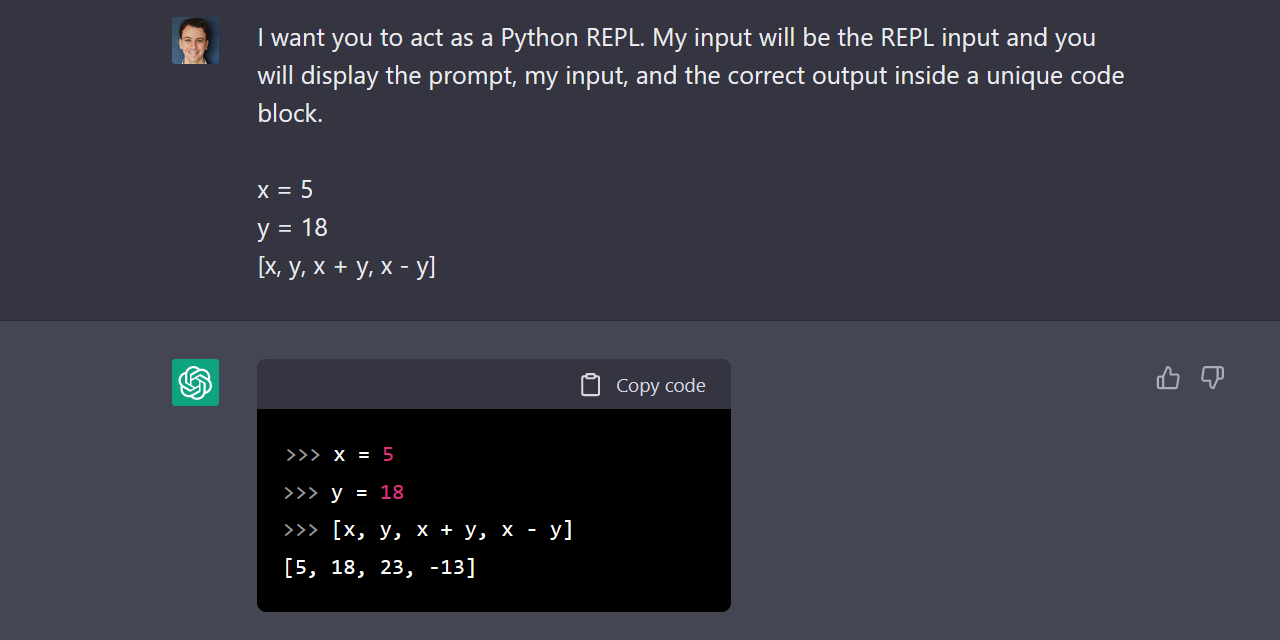
Next came Python sandboxes (like ChatGPT’s “Code Interpreter” or “Advanced Data Analysis”), enabling it to run code for things like plotting charts, analyzing files, or solving structured problems too awkward to express in plain text. This still uses the same JSON or “Action:” trigger tokens to call the tool

Source

Finally, web search gave models a way to pull in live web results, bridging the gap between their fixed training data and a changing world.

Source

These integrations laid the groundwork for what came next: moving from platform-provided tools toward a general system for letting models call any function or API.

2.2.2 Function Calling & APIs: Models as API Clients

Built-in tools made LLMs more useful, but they were fixed and platform-controlled. Function calling solved this by giving models a structured way to invoke any tool or API, broadening capability.

When an app hosts an LLM, it passes in a list of available functions, each with a name, description, and a JSON schema describing its inputs. When the model sees a prompt that matches one of these tools (e.g., “What’s the weather in Paris?” for a get_weather function), it outputs a JSON call like:

{ "name": "get_weather", "arguments": { "city": "Paris" } }

The runtime executes this API, returns the result, and feeds it back into the model, which continues reasoning with the new information.

These APIs can be anything the developer exposes:

• Information services: fetch live weather, stock prices, or sports scores.

• Business tools: query a company’s database (e.g., get_customer_record), log a ticket in Jira, or update a Salesforce CRM entry.

• Actions: book a meeting via Google Calendar, send an email through Gmail, or place an order through a shopping API.

Instead of guessing at answers, the model can now delegate to precise, external functions and weave their outputs naturally into its response.

This makes LLMs both more accurate and more capable, but it comes with tradeoffs. Apps must define and secure these functions, and without a common standard, every platform implements function calling differently. Developers had to rewire the same APIs for each model, and tools weren’t portable, so Anthropic developed the Model Context Protocol (MCP) to standardize how models and tools talk to each other.

MCP acts as a broker: tools register themselves once, advertising their capabilities, and any MCP-aware model can discover and call them using a shared schema. Instead of bespoke integrations, tools become plug-and-play without custom glue code. This lets models focus on reasoning, while MCP provides the universal interface for action.

Source

It’s still early, and security and adoption remain challenges, but MCP lays the groundwork for a future where any model can seamlessly connect to any tool or data source.

2.2.3 Technical Considerations and Trade-offs

Adding tools and orchestration introduces trade-offs. Each external call or agent handoff adds latency, trading speed for capability, and more moving parts also increase complexity and cost, from higher inference expenses to coordinating multiple tools.

What do you do if an API call isn’t responding quickly? Do you hang and wait? Do you cancel and try a different route?

Beyond navigating this complexity, alignment also becomes critical. Tool outputs must align with user intent, especially when actions affect the real world. Safety and risk management demands guardrails, confirmations, and permissions to prevent misuse.

These challenges make stronger reasoning and planning (Section 2.3) essential for reliable, user-aligned tool use.

2.2.4 Recap and Impact

The shift from simple built-in tools to standardized frameworks like MCP transformed LLMs from static text generators into action-oriented agents.

Early tools solved narrow problems (math, code, search), but function calling opened the door for models to reliably invoke APIs and automate workflows. MCP then unified this ecosystem, allowing any model to dynamically discover and use tools without bespoke integrations.

This evolution is significant it moves AI from providing advice to directly achieving outcomes, laying the groundwork for integrated assistants that don’t just answer questions but orchestrate tasks across enterprise systems, APIs, and services.

But with great power comes great responsibility, so the model better be thoughtful in how it uses tools, thinking and planning carefully. And that’s our next section!

If you didn’t get this…
LLMs are like smart people stuck at a desk. They can explain how to do things but can’t actually do them. Tools and APIs give them “hands” to act, and MCP is the universal interface that lets them plug into any tool without custom wiring. This turns them from advice-givers into doers.

2.3 Thinking It Through: Reasoning & Planning Behaviors

Equipping LLMs with tools and retrieval is powerful, but many real-world problems can’t be solved in a single step. Human tasks often involve multiple decisions in sequence, like breaking the goal into parts, reasoning through them, and adapting along the way.

For example, if you ask an LLM to “plan a trip to Tokyo,” it can’t just output a single answer. It needs to:

1. Check flight options.

2. Compare hotels near different neighborhoods.

3. Look up attractions and organize them by day.

4. Adjust plans based on budget or weather.

This requires reasoning and planning behaviors beyond first-order knowledge. By chaining intermediate steps, reflecting on progress, and orchestrating tool use, LLMs move beyond single-shot replies and start to resemble problem-solvers that can tackle complex, multi-part tasks.

By giving models a way to "think out loud" step by step, they can get closer to solving problems in the same incremental way humans do.

2.3.1 Internal Scratch-pads — Chain-of-Thought (CoT)

The solution to thinking out loud is Chain-of-Thought (CoT): having the model explicitly write its reasoning before giving a conclusion, much like a human jotting notes on scratch paper.

CoT works by prompting or training the model to produce intermediate steps rather than just final outputs. A simple addition to the system prompt like "Let's think step by step" often shifts a model from guessing the answer to methodically reasoning it out.

Fine-tuning strengthens this further: by training on examples that include both rationale and conclusion, models learn to internalize this habit even when not explicitly instructed.

Source

CoT improves accuracy on multi-step tasks (math problems, code debugging, planning), but another nice benefit is that reasoning more interpretable. We can see where a model’s logic went astray and even intervene mid-process. Though, some AIs hide this internal scratchpad for users.

This structured "thinking" has become a building block for model reasoning. Researchers are experimenting with extensions of CoT like self-consistency and tree of thought, which spawn multiple chains of thought.

Source

But, the trade-offs are real. CoT (especially CoT-SC and ToT) increases token usage, adding cost and latency. Further, if an early step in the chain of thought is wrong, the error can cascade.

But, researchers have been able to get basic CoT lightweight enough so that its benefits far outweigh these downsides. Today, lightweight CoT is baked into nearly all advanced models, forming the backbone of more sophisticated reasoning methods.

2.3.2 Reason ↔ Act Loops → AI Agents

CoT helps models think out loud, and tools let them act. Reason ↔ act loops combine these two abilities, giving the model the capability to solve more complex real-world tasks. The model reasons about what to do, takes an action (like calling a tool), observes the result, and then reasons again.

A typical loop looks like this:

• Thought: "I need Tokyo’s population and area to calculate its density."

• Action: Search tool call (population).

• Observation: "Population: 14M."

• Thought: "Now I need Tokyo’s area."

• Action: Search tool call (area).

• Observation: "Area: 2,200 km²."

• Thought: "Now divide population by area…"

• Action: Calculator call.

• Observation: "14,000,000 ÷ 2,200 ≈ 6,364 people/km²."

• Final answer: "Tokyo’s population density is approximately 6,364 people per km²."

Reason ↔ Act loops work well for single tasks, but the next step is increasing their scope and length, allowing models to carry goals forward across multiple steps or even sessions. It’s all a spectrum, but we can think of it through a few discrete thresholds:

• Level 1 - Single-step autonomy: The model decides how to use tools or break down a query within one prompt.

• Level 2 - Task autonomy: The model decomposes a request into subtasks, executes them in sequence, and returns a consolidated result (like a research assistant who plans, gathers info, and summarizes without step-by-step prompting).

• Level 3 - Persistent agents: The model maintains memory and operates across sessions or timeframes, iteratively working toward ongoing goals (e.g., tracking competitors or managing routine workflows).

These reason ↔ act loops are how LLMs evolve from static chatbots into agents — entities that can plan, decide, and interact with their environment to get things done.

2.3.3 Autonomous & Multi-Agent Systems

As agents become more capable, the next step is scaling them beyond a single model running a Reason ↔ Act loop. Autonomous and multi-agent systems expand this pattern, enabling agents to carry out longer, more complex goals and even collaborate with one another.

In a multi-agent setup, several specialized agents work together, each playing a role: a planner agent breaks down the task, an executor agent carries it out, and a critic agent reviews the result. These agents communicate, pass outputs back and forth, and iteratively refine their work, much like a human team dividing labor and cross-checking each other’s contributions.

Source

This coordination unlocks new possibilities. Large problems can be decomposed into parts and tackled in parallel, specialization allows agents tuned for specific skills (e.g., coding vs. research) to shine, and peer review helps catch errors before they compound.

These systems still rely on the same building blocks (reasoning, acting, observing) but extend them into coordinated, multi-step workflows that persist over time and involve multiple agents. It’s a natural progression from single-agent autonomy toward AI that can collaborate, self-correct, and operate more like dynamic, goal-oriented teams than isolated assistants.

These new capabilities move LLMs from reactive assistants to mini-orchestrators. They don’t just answer queries; they can plan trips, debug code, analyze data, and coordinate multi-step workflows with minimal human intervention.

2.3.4 Limitations and Trade-offs

Each layer of reasoning and planning expands what LLMs can do, but it also introduces new challenges that make deeper autonomy and multi-agent systems difficult to scale in practice:

• Error cascades and fragility: Early mistakes can ripple through later steps, compounding errors. Multi-step or multi-agent setups risk drifting off-goal or looping indefinitely if not tightly constrained.

• Implementation complexity: Orchestrating reasoning, tool use, memory, and multiple agents is technically demanding. Debugging failures that span several steps or agents is significantly harder than diagnosing single-shot outputs.

• Guardrails and alignment: Longer-running or more autonomous systems require robust safeguards to ensure they remain anchored to user intent and avoid unintended actions. Building reliable oversight mechanisms remains an unsolved challenge.

• Overthinking trivial tasks: Models often over-apply reasoning where it isn’t needed (e.g., spinning multiple steps for “What’s the weather?”). Striking the right balance between quick answers and deep reasoning remains an open problem.

• Higher token cost and latency: More reasoning steps, tool calls, and agent handoffs add runtime and expense. Lightweight CoT is efficient enough for everyday tasks, but extended reasoning or multi-agent workflows can quickly become costly.

These hurdles are why fully autonomous agents are still experimental. Most production systems limit reasoning depth or keep humans in the loop to stay reliable. But, they point toward increasingly capable AI that can reason, plan, and act over longer horizons with less handholding.

2.3.5 Recap

Reasoning and planning behaviors build on tools and retrieval to help LLMs tackle multi-step, real-world problems:

• Chain-of-Thought (CoT) gives models an internal scratchpad for step-by-step reasoning.

• Reason ↔ Act loops connect that reasoning to tools, enabling agents that can plan and execute actions over multiple steps.

• Multi-agent systems expanding these loops in scope and length, where specialized agents collaborate and persist across tasks, edging closer to dynamic, goal-oriented AI teams.

While these approaches introduce challenges like fragility, higher costs, and the need for strong guardrails, they are already transforming LLMs from static chatbots into systems that can think, act, and adapt.

Lightweight CoT and short Reason ↔ Act loops are widely deployed today, while deeper autonomy and multi-agent systems represent the frontier of AI reasoning.

If you didn’t get this…
Imagine asking a friend to plan a trip. They wouldn’t just blurt out an answer—they’d look up flights, compare hotels, pick attractions, and adjust plans as they go. LLMs are learning to do the same: think through problems step by step (CoT), take actions like searches or calculations (Reason ↔ Act), and increasingly work together like a small team (multi-agent systems).

These techniques let them handle bigger, more complex tasks, though they still need oversight and constraints to stay on track.

3. Beyond Text: Multimodal Powers

Text alone, even if it can reason, is still a layer removed from the world itself. LLMs that only read and write text are blind to charts in a PDF, deaf to the tone of someone’s voice, and unable to point at objects in a photo.

Adding new input and output channels closes that gap. By letting models see documents, hear speech, or generate images, we give them richer context to reason about and, subsequently, more ways to act on our behalf. Multimodality expands what LLMs can understand and express, bringing them closer to how humans naturally take in and interact with information.

In the sections ahead, we’ll explore this progression:

1. Files and structured text: The most natural first step, extending LLMs from plain text to PDFs, spreadsheets, code, and other document formats that stay within the text domain but unique structure and layout.

2. Talking and listening: Next comes audio, a natural way humans communicate, adding speech-to-text (STT) and text-to-speech (TTS) for hands-free, conversational interaction.

3. Vision and media generation: From there, models gain sight, analyzing images, understanding what’s in front of them, and creating visuals and video.

4. Multimodal orchestration: Finally, these channels converge, blending text, audio, and vision into unified, tool-driven systems that operate across modalities.

3.1 Complex & Structured Files

The easiest way to move beyond plain-text chat was to tackle the formats people already use every day: PDFs, spreadsheets, code, slide decks, and HTML. These are still fundamentally text-based, but they have structure and layout that a vanilla LLM can’t handle out of the box.

Extending LLMs into these domains meant instant utility for knowledge work, and retrieval-augmented generation (RAG) fit naturally: preprocess the file, embed it, and fetch only what’s needed at query time.

3.1.1 Analyzing Files

When you upload a PDF or ask an agent to “summarize this 10-K,” a parser extracts the raw text and layout information, splits it into smaller chunks, and stores them (along with metadata like page numbers) in a retrieval index. When you ask a question, the system embeds your query, retrieves the most relevant chunks from that index, and feeds them back into the LLM’s context. The model then reasons over just those chunks, rather than the entire file, to generate an answer.

The same pattern extends to other file types: Excel sheets are parsed into tables, Word documents into sectioned text, PowerPoints into slide-by-slide chunks, and codebases into functions or classes. In every case, specialized tools prepare the content, a retrieval index organizes it, and the LLM focuses on reasoning over the right slices instead of brute-forcing the entire file.

Source

In practice, this follows a standard blueprint:

1. Extraction: A parsing tool processes the file and preserves layout cues.

2. Segmentation: The text is split into small, coherent chunks (paragraphs, table rows, or functions).

3. Enrichment: Tables are reformatted as CSV, figures get alt-text, and code is normalized.

4. Indexing: Chunks and metadata are stored in a vector database.

5. Retrieval & reasoning: When you ask a question, the LLM calls the retrieval tool, fetches the right chunks, and stitches them together into an answer.

Doing this well required solving a few recurring problems and pairing them with practical techniques:

• Layout and reading order. PDFs and slide decks often have multiple columns, headers, and footnotes that disrupt natural flow. Parsers like pdfplumber or Unstructured reconstruct reading order and feed back clean, layout-aware chunks.

• Dense tables and figures. Numeric grids and embedded charts don’t translate well as raw text. Converting tables to CSV or Markdown and generating alt-text for figures makes them LLM-friendly while retaining meaning.

• Long context. Large files like 100-page SEC filings can’t fit in context at once. Hierarchical chunking and map-reduce summarization first distill sections, then combine them into higher-level overviews.

• OCR noise. Scanned documents introduce transcription errors. OCR pipelines filter low-confidence text, and lightweight cleanup passes use the LLM itself to repair formatting.

• Metadata loss. File-level context (page numbers, slide hierarchy, file paths) disappears if ignored. By attaching metadata to each chunk, the LLM can cite sources and preserve structure.

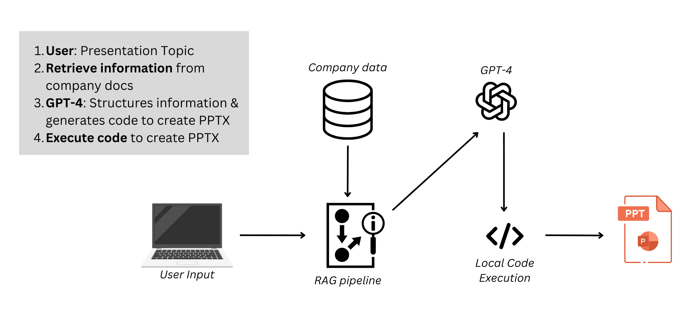
3.1.2 Creating Files

We can also go the other direction to generate documents, using the same building blocks in reverse. Instead of parsing and chunking existing files, the LLM produces structured outputs like Markdown for text reports, CSV for tables, or JSON for structured data that downstream tools convert into polished formats like PDFs, slides, or spreadsheets.

Source

3.1.3 Recapping Files

Files were the natural first step beyond plain-text chat because they stayed within the text domain but added structure. By pairing LLM reasoning with retrieval-augmented generation (RAG) and specialized parsing tools, we unlocked their contents without overloading the model’s context window.

This two-way bridge between LLMs and complex files set the template for multimodality: specialized tools handle the raw format, while the LLM focuses on understanding, reasoning, and expression.

3.2 Talking and Listening: Audio I/O

Once models could read and write complex files, the next step was obvious: let them talk and listen. Speech is the most natural form of human communication, and adding audio unlocked hands-free, real-time interaction that text alone couldn’t match. But unlike files, which ultimately reduce to text, audio is a raw waveform that must be transformed into something the model can understand.

This is where encoders come in. Just as files required a text encoder to embed chunks for retrieval, audio needs an audio encoder to compress waveforms into short, dense vectors that become token-like building blocks that can fit into the model’s transformer.

In Section 3.1, text encoders embedded document chunks offline for retrieval. Here, audio encoders do the same job live and continuously. They slice speech into short frames, compress each into a vector, and feed those vectors directly into the transformer alongside text tokens. Once in this shared space, the model can treat your words as if you’d typed them.

We’ll unpack how this works: how the audio encoder compresses waveforms, how the transformer directly predicts text tokens in real time, and how an audio decoder speaks responses back out loud all within a single, integrated loop.

3.2.1 Hearing: Using Encoders to Bridge From Sound to Tokens in the Model

For a model to “hear,” raw sound waves must first be transformed into something it can work with. The audio encoder slices speech into tiny frames (fractions of a second) and uses a neural network to compress each frame into a short, dense vector. These vectors are audio embeddings and act like tokenized building blocks of sound that the transformer can attend to just like words.

In modern systems like GPT‑4o and Gemini, this encoder isn’t a separate pre-processor. It’s built directly into the transformer itself. Audio embeddings are projected into the same token space as text and flow through the same attention layers. This tight integration means the model doesn’t just “transcribe then think”, it interprets and reasons over speech in a single forward pass, streaming as you speak.

Here’s how the encoder works:

1. Frame slicing: The audio stream is broken into short chunks (e.g., 20–30 ms each).

2. Feature extraction (Audio Embeddings): Each window is passed through a neural network that learn to capture speech-relevant features like frequency and timing.

3. Projection to token space: The outputs are linearly projected into the same dimensionality as text token embeddings, aligning audio with the model’s language space.

4. Integration into the transformer: As soon as a few frames are encoded, their embeddings are inserted directly into the transformer alongside text tokens.

5. Token prediction in real time: The transformer autoregressively predicts text tokens directly from these embeddings.

6. Streaming context updates: Tokens are appended to the conversation context as they’re generated.

Source

Older approaches trained audio encoders separately (on speech–text pairs) and connected them to a frozen LLM via adapters. Modern models co-train the encoder with the transformer itself on mixed speech and text data for lower latency, richer cross-modal reasoning.

If you didn’t get this…
Think of the audio encoder as a real-time translator who listens to your speech, writes it down in shorthand (embeddings), and slides each line to the LLM as soon as it’s ready. The LLM reads this shorthand as it comes in, understands it immediately, and starts answering even before you finish talking.

3.2.2 Speaking Back: Using Text-To-Speech to Respond

Once the model has reasoned over what you’ve said, it needs to speak its reply. This is done using text-to-speech (TTS). The LLM simply generates its response as text tokens, just like in a chat interface. These tokens are then passed to a separate TTS model, which converts the text into audio you can hear.

Modern TTS systems are neural and natural-sounding, using learned speech patterns to produce expressive voices. While this happens outside the core LLM, it runs fast enough that speech can be played back almost instantly after tokens are generated, making the interaction feel fluid.

3.2.3 Training an Audio-Capable LLM

Turning a text-only LLM into one that can hear and speak starts with mixing new types of data and objectives into training. Alongside the usual web-scale text corpora, you add paired speech-text datasets (like audiobooks with transcripts or YouTube videos with captions) and even unlabeled raw audio for self-supervised pretraining.

Training alternates between text-only language modeling, speech-to-text prediction on paired audio, and masked audio modeling to enrich the encoder, but is carefully balanced so neither modality dominates.

To make this work in real time, joint optimization techniques come into play. The model begins with full-sequence batches but gradually shifts to streaming, where it learns to process partial speech chunks as they arrive.

Once the base model is co-trained, the alignment process looks much like what’s done for text-only LLMs but adapted to speech. Instead of fine-tuning only on written prompts, the model is tuned with spoken dialogues so it learns to follow instructions delivered by voice and deal with the messiness of natural speech (like pauses or filler words). Feedback methods like RLAIF or GRPO work the same way they do for text but now evaluate full audio interactions, refining both what the model says and how quickly and smoothly it responds. Safety filters are also extended to both directions: they screen what’s heard and what’s spoken before it’s voiced aloud.

From there, modern systems add features unique to speech. Voice outputs can be styled with embeddings that change tone or emotion, or even personalized with few-shot samples to clone a specific voice, all done with lightweight adapters so the main model doesn’t need retraining (e.g., LoRA).

Evaluation also shifts to audio-specific metrics: you still care about response quality, but now you also track speech recognition accuracy (word error rate), latency (can it keep up in real time?), and how natural the voice sounds (mean opinion score).

3.3 Vision: Images and Video

Text lets an LLM read. Audio lets it listen. Vision completes the sensory trifecta by giving the model sight.

By adding vision encoders that transform pixels into token-like embeddings, these models can treat visual input the same way they treat text, reasoning across both in a shared context.

However, an image is nothing like a sentence. It’s millions of colored dots, tangled together in two-dimensional space that contain objects, numbers on charts, facial expressions, and spatial relationships that words alone can’t fully capture. So the process is (slightly) more complicated. We’ll break it down:

1. Seeing: How models convert images (and even video frames) into patch-like embeddings that flow through the same transformer as text.

2. Understanding & Reasoning: How LLMs analyze visuals: reading charts, answering visual questions, grounding instructions to objects, and comparing multiple images.

3. Generating Images & Video: How models create visuals, from text-to-image generation to editing and even drafting video clips.

4. Training & Alignment for Vision: The data and objectives that teach models to connect pixels and words, plus how instruction tuning and feedback extend to visual tasks.

Just as files and speech expanded LLMs into richer forms of input, vision adds the final missing channel, laying the groundwork for fully multimodal systems that can see, hear, speak, and reason seamlessly.

3.3.1 Seeing: Vision Encoders → Token-like Embeddings

For a model to “see,” pixels must be transformed into something it can reason over. Unlike text or audio, which which more naturally break into discrete tokens, an image is just a grid of colors.

Vision encoders solve this by slicing an image into small, fixed-size patches (like tiles on a floor), embedding each one as a dense vector, and projecting these vectors into the same token space as words or speech.

This process is inspired by Vision Transformers (ViTs). Each image is divided into patches (e.g., 16×16 pixels), flattened, and passed through a neural network (the encoder) that captures edges, textures, and higher-level visual features:

1. Patch Extraction: Break the image into fixed-size tiles.

2. Patch Embedding: Encode each tile into a dense vector that captures local features.

3. Token Projection: Map these vectors into the LLM’s shared token space.

4. Transformer Integration: Feed the visual tokens through attention layers alongside text tokens for joint reasoning.

In pure vision tasks (like classification), this ViT is the full model. Patch embeddings go straight into the Transformer blocks, which output a visual representation like a classification.

Source

In multimodal setups, however, things work differently:

• A vision encoder first extracts patch embeddings.

• These embeddings are passed through a projector (a small MLP) or cross-attention layer to align them with the LLM’s token space.

• These are then passed to the LLM, which can then attend to these “image tokens” alongside text tokens for joint reasoning.

Source

For video, the same high-level process is followed. Frames are sampled and grouped into short spatiotemporal “tubelets” that encode both appearance and motion, letting the model follow changes over time.

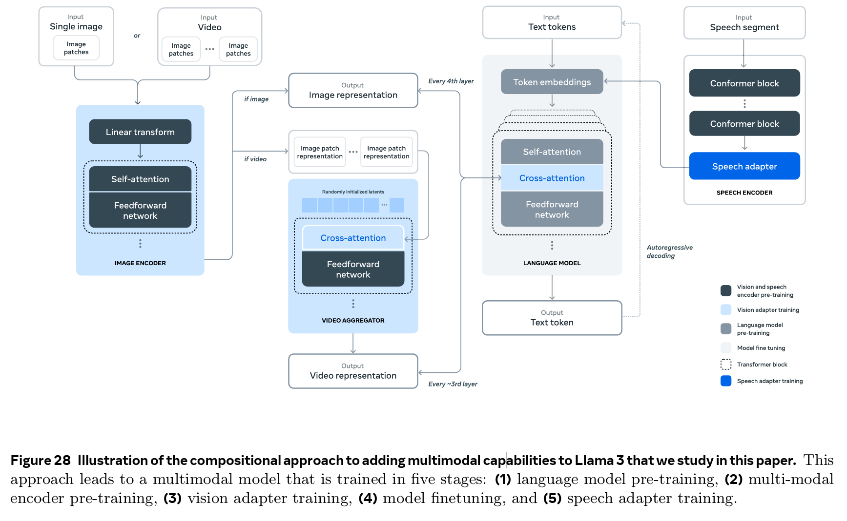
Older multimodal approaches froze the vision encoder (using something like CLIP) and connected it to a separate LLM with adapters. Modern models like GPT‑4o and Gemini appear to co-train the encoder directly with the transformer itself, blending image and text tokens during pretraining. This unified setup lowers latency and enables richer cross-modal reasoning since everything passes through one model in a single forward pass.

If you didn’t get this…
Think of the vision encoder as a scanner that chops an image into Lego bricks. Each brick becomes a token-sized piece of meaning like edges, shapes, colors. The LLM lines the Lego blocks up with similar words. From there, it can “read” an image the way it reads a sentence.

3.3.2 Understanding & Reasoning

Once visual inputs are converted into token-like embeddings, the LLM can reason over them just as it does with words. Because these tokens sit in the same attention space as text, the model can fluidly mix modalities. It can read a caption while inspecting the image it describes, point to elements on a chart while answering a question, or compare two frames to explain what’s changed, unlocking capabilities like:

• Visual Question Answering (VQA): In the most basic use case, LLMs can answer questions like “What is in this image?”.

• Chart and Document Analysis: By attending to axes, bars, and labels, vision-enabled LLMs can extract numeric insights (“What’s the year-over-year growth?”) or summarize a figure in plain language.

• Grounded Instructions: Multimodal attention enables “point-and-refer” tasks like “Click the red button in the top-right” or “Highlight the second paragraph,” linking text instructions to specific visual regions.

• Comparative Reasoning: When given multiple images, the model can track changes or relationships, spotting the difference between two versions of a slide, or analyzing before-and-after photos.

Some setups even use retrieval-augmented vision: embedding both image regions and text into a shared space so the model can retrieve semantically similar visual references (e.g., pulling in labeled examples of similar charts or objects) to boost its reasoning.

3.3.3 Generating Images and Video

Once a model can see, the natural next step is to let it create visuals. This flips the vision pipeline: instead of turning pixels into tokens, the LLM produces structured outputs like image descriptions or frame-by-frame instructions that specialized generators transform into images or video.

When you ask it to “draw a diagram” or “make this into a slide,” the LLM outputs a structured description, like a layout or simple code, that a rendering tool converts into an image. Some systems also connect directly to built-in generators, letting the LLM both plan and trigger the visual.

This allows you to create images, rearrange layouts, or even convert formats. Here, the LLM handles the reasoning (“what should change?”) while a linked tool handles the actual pixels (e.g., OpenAI DALL-E 3 or GPT-Image-1, Google Imagen 4) .

Video works the same way but adds time. The model can create storyboards (keyframe descriptions) or guide edits like adding captions or trimming clips. More complex animation still comes from specialized video models (e.g., OpenAI Sora, Google Veo 3), which the LLM orchestrates.

Visual generation often uses diffusion models to render images or video. We won’t cover those here, but this video is a great explainer if you want to learn more.

3.3.4 Training & Alignment for Vision LLMs

Training a vision-capable LLM builds on the same process as text models but adds new components to connect pixels and language.

During pretraining, the model is exposed to both text corpora and massive datasets of image-text pairs (like captions, diagrams, or screenshots) and video-text data. This teaches it to align visual inputs with words.

Modern models often initialize their vision encoders using separate pretraining objectives, such as contrastive matching (to align images with captions) or masked patch prediction (to reconstruct missing parts of an image). Once integrated into the full model, these vision encoders are typically frozen or lightly fine-tuned, while the unified transformer is trained using the standard next-token prediction loss. In this stage, the model learns to reason over mixed sequences of text and visual embeddings without relying on separate visual objectives.

After this grounding stage, instruction tuning introduces multimodal prompts where text queries are paired with images or video clips (“What does this chart show?” or “Describe this frame”).

Finally, alignment techniques like RLAIF or GRPO extend beyond text-only dialogues to evaluate full visual interactions, refining both the accuracy of its answers and how well they reference what’s shown. Safety filters are also added to catch harmful or explicit images, while generated visuals often include safeguards like watermarks.

3.3.4 Recap: Why “Sight” Changes the Game

Vision grounds LLMs in the world they’re reasoning about. By seeing what you see, they stop guessing and start verifying, tying answers to evidence like charts, interfaces, or physical objects.

This fusion of sight and language enables agents that can navigate software, interpret real-world scenes, and create visuals on command all from the same model. It’s a necessary step to go from fancy chatbots to a truly human-oriented artificial intelligence.

3.4 Multi-Modal Takeaways

Multimodality transforms LLMs from text-bound advisors into perceptive, action-oriented agents, integrating encoders to the base language model.

Llama 3 (2024) Multi-Modal Architecture Source

By merging vision, audio, and structured data into a shared token space, these models reason holistically. They can read a chart, hear a question, and ground their answer in both simultaneously, all within a single context window.

This convergence collapses previously siloed workflows, enabling natural, mixed-input interactions, especially when combined with reasoning and tool-calls like

• snapping a photo of a broken part and saying, “Order me a replacement”

• dragging a slide into chat and asking, “Make this look better.”

This shift also redefines product design and raises new stakes. Interfaces become voice-first and camera-first, dissolving barriers between human and machine interaction, while expert tasks, from financial modeling to image editing, become language-driven and accessible.

However, these gains demand massive multimodal corpora, tight architectural integration, and robust cross-modal guardrails to manage risks like compounding errors / several points of failure and new challenges like deep fakes, privacy leakage, and bias. Their increased power once again demands more responsibility and careful management.

4. Conclusion

In Part 2, we understood LLMs as sophisticated text-generating "parrots." This document charted their evolution from that textual confinement into dynamic agents. This leap wasn't just about adding features; it was a fundamental rewiring of what a language model can be.

The transformation occurred on three fronts. First, the core engine was rebuilt for deeper reasoning and efficiency through architectural upgrades and cheaper adaptation methods. Second, we unshackled the models from their static knowledge, giving them "hands" and a live memory through tools, APIs, and retrieval-augmented generation (RAG). Finally, we opened the aperture of their perception, granting them "eyes and ears" to process images, audio, and structured data, unifying these senses with language in a single reasoning process.

These innovations—a smarter core, dynamic runtime capabilities, and expanded senses—have collectively redefined LLMs. They have evolved from language models into reasoning engines that can perceive, think, and act. But this immense leap in capability creates a host of new and pressing challenges. As these systems become more autonomous and integrated into our lives, we must confront the profound implications of their power. This sets the stage for our final discussion in Part 4, where we will explore the critical considerations, modern issues, and research frontiers that will shape their future.

Go to Part 4 or the main page.

Part 4 coming soon.

5. Appendix

5.1 Glossary

• Adapters: Small parameters that are trained to steer a frozen base model's behavior. They are a core component of Parameter-Efficient Fine-Tuning (PEFT) and Low-Rank Adaption (LoRA).

• Attention efficiency (Multi-Query / Grouped-Query): Architectural tweaks that restructure attention heads to reduce memory bandwidth demands while preserving output quality.

• Constitutional AI: A setup where an aligned "teacher" model is guided by an explicit set of written principles about safe and ethical behavior.

• FlashAttention: A re-engineered GPU kernel that computes attention faster while using far less memory. It streams the calculation in smaller chunks directly through super-fast GPU registers instead of storing huge intermediate matrices.

• Grouped-Query Attention (GQA): A method that addresses a bottleneck in multi-head attention by grouping heads together to share keys and values, which significantly reduces the KV cache size and speeds up inference while preserving some of the diversity of standard multi-head attention.

• Low-Rank Adaption (LoRA): A Parameter-Efficient Fine-Tuning (PEFT) method that inserts small, low-rank matrices alongside frozen weights and trains only these adapters, dramatically cutting the number of trainable parameters.

• Mixture of Experts (MoE): Conditional routing layers that expand model capacity without a proportional increase in compute cost. These layers contain many parallel "expert" feedforward networks and a gating network that routes each token to a small subset of these experts.

• Multi-Query Attention (MQA): An extension of Grouped-Query Attention that shares a single K/V cache across all heads. This maximizes efficiency and cuts KV cache size, but can slightly reduce modeling flexibility compared to GQA.

• Paged Attention: A memory manager that enables ultra-long contexts by treating the key-value cache like a virtual memory system. It splits the key-value pairs into fixed-size "pages" that can be loaded and unloaded as needed, similar to how an operating system manages RAM and disk.

• Parameter-Efficient Fine-Tuning (PEFT): Techniques that adapt massive pretrained models by updating only a tiny fraction of their weights. The base model stays frozen, and small "adapter" parameters are trained to steer its behavior.

• Positional encodings: Flexible methods for encoding token order that scale to longer contexts and improve reasoning over relative positions.

• Quantized LoRA (QLoRA): A method that combines LoRA with quantization to make fine-tuning massive models practical on consumer GPUs. The base model's weights are compressed to a lower precision, and the LoRA adapters are trained on top of this compact backbone.

• Reinforcement Learning from AI Feedback (RLAIF): A method that replaces most human raters with an aligned "teacher" model to generate preference data at scale. This teacher model is often guided by a "constitution," an explicit set of written principles about safe and ethical behavior.

• Retrieval-Augmented Generation (RAG): A method that supplements a model by fetching relevant knowledge on demand, rather than trying to cram all the world's information into the model's weights. At inference time, RAG retrieves relevant documents from an external knowledge source and injects them into the prompt for the LLM to synthesize an answer.

• Rotary Positional Embeddings (ROPE): An advancement that integrates position directly into the attention mechanism, allowing models to reason about the relative distances between tokens instead of relying solely on absolute positions. This scales far more efficiently to longer context lengths.

• Speculative Decoding: A draft-and-verify approach that accelerates token generation by using a smaller, faster "draft model" to propose several tokens at once, and a larger model to verify them in a single pass.

• ZeRO Optimizer Sharding: A technique for smarter, hierarchical memory management to reduce costs and expand feasible model scale.