A Semi-Technical Primer on LLMs: Pt. 2 From Model to Chatbot

Understanding how applications like ChatGPT are structured, trained, and made useful.

In Part 1, we explored how models learn by example, using labeled data to map inputs to outputs. But since labeling data is slow and costly, we introduced a powerful shortcut: self-supervised learning, which turns raw data itself into training labels. Paired with embeddings — compact representations that capture meaning and relationships — this approach enabled models to understand and reuse patterns across countless tasks.

But to make the leap from simple tasks to the sophisticated, general-purpose language models we see today, researchers needed an architecture that could scale effectively. That’s where the Transformer architecture comes in.

Transformers were designed to generate text by predicting the next token in a sequence, relying on just a few elegantly simple building blocks stacked in layers. The approach worked incredibly well, particularly when researchers adopted a two-step training process:

• Pre-Training: The model learns general language patterns from massive datasets, forming a strong foundation.

• Post-Training (Fine-Tuning): The model specializes to handle specific tasks with greater accuracy.

That’s why they called it the Generative Pre-trained Transformer (GPT) — a model designed to generate language, pre-trained on massive datasets before fine-tuning, using the Transformer architecture.

Yep, that’s the GPT in ChatGPT! Now that we know how it got its name, let’s take a look under the hood to see how it works. We’ll cover:

1. The Architecture — How the algorithm in the model works

2. Training — How feeding data through to make it smart

3. Inference — How the model produces outputs once it has been trained

4. Evaluation — How we measure whether the model is actually useful, safe, and aligned with human goals

Let’s dive in!

Naturally, there is a bit of jargon in here. To help navigate this, words in bold are defined / clarified in a glossary at the end of each part.

1. The GPT Architecture

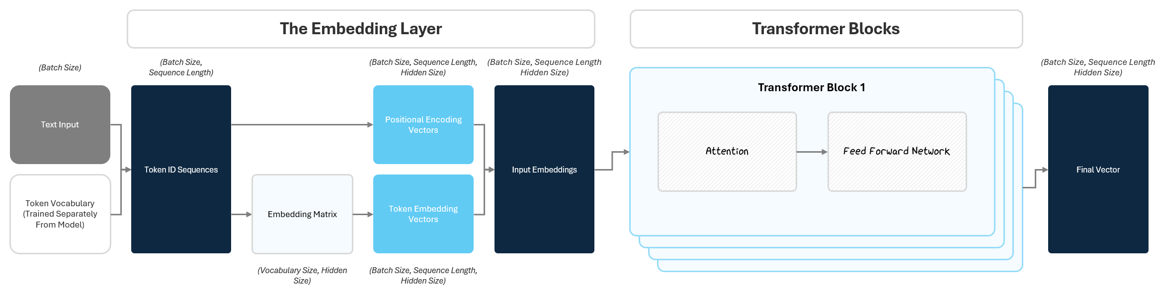
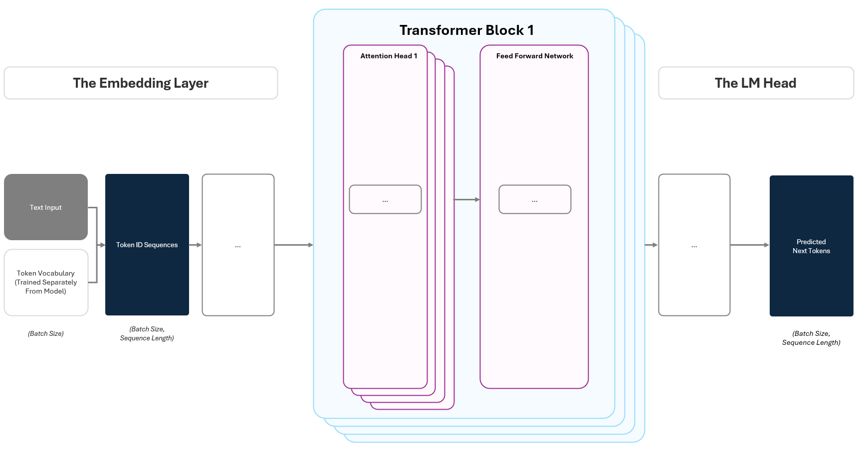
At its core, the GPT architecture is made up of three main components:

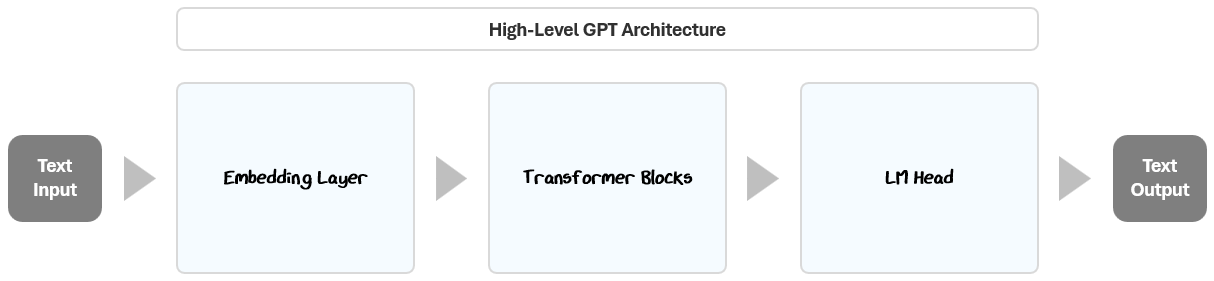
• Embedding Layer: Converts raw text into numeric vectors that capture meaning and context.

• Transformer Blocks: Analyze and refine these embeddings to recognize important relationships and patterns in language.

• Language Model (LM) Head: Uses these refined vectors to predict the most likely next word in a sequence.

Together, these components enable GPT to process input text, learn from patterns, and generate coherent responses.

Let’s break each of these down, starting from the very beginning: the Embedding Layer.

1.1 The Embedding Layer: From Raw Text to Context-Rich Vectors

Before a model can understand language, it needs a way to translate raw text into something numerical — our neural networks from Part 1 can’t take the dot product of text — and meaningful. This is exactly what embeddings accomplish. Embeddings are like coordinates on a vast map of meaning. They convert each piece of text into compact numerical vectors that represent context, meaning, and usage.

In the embedding examples below, we can see how in the graphs, words of similar meaning have similar coordinates.

Source

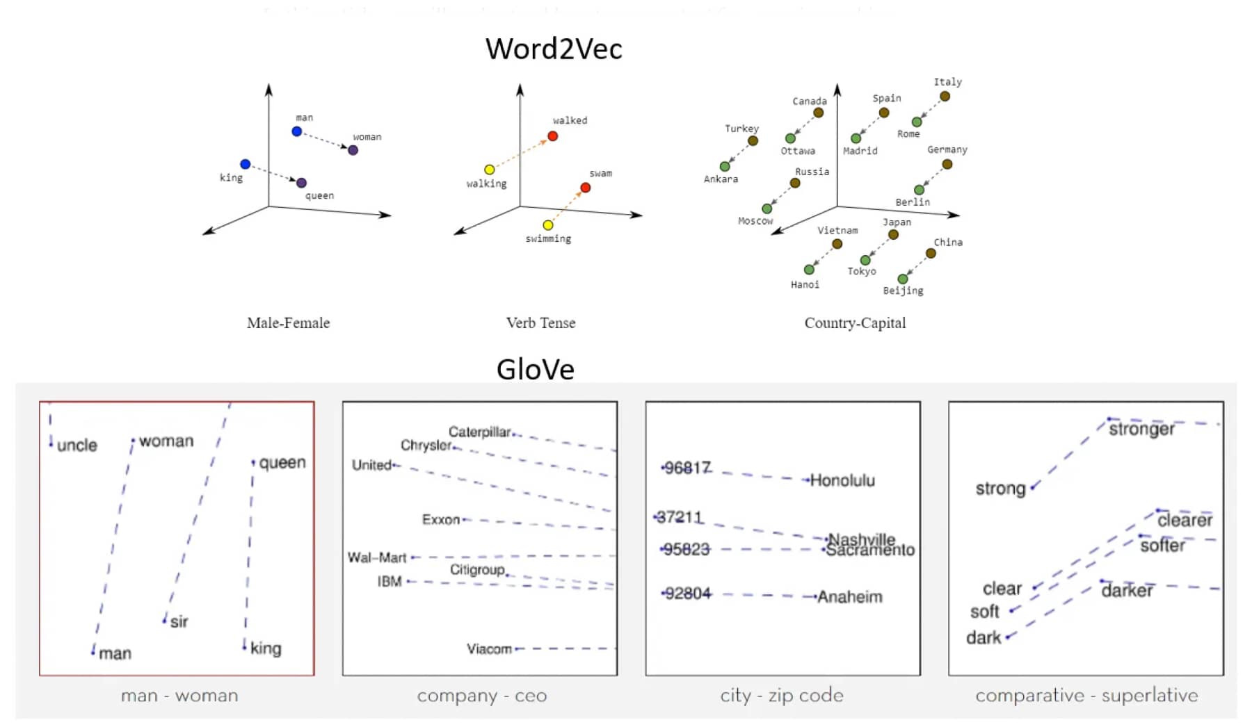
Once translated into these embeddings, words and tokens become mathematical objects the model can process and analyze.

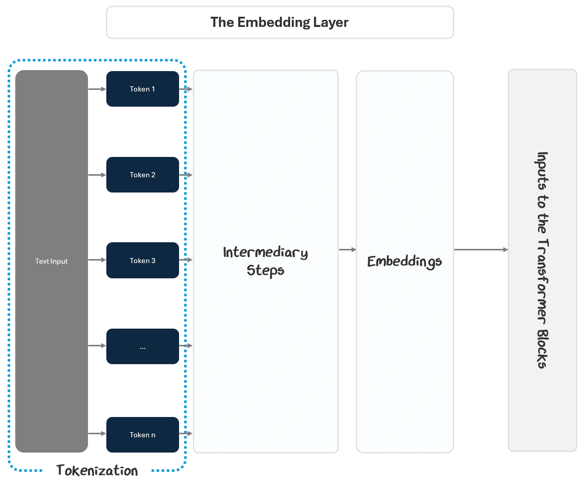
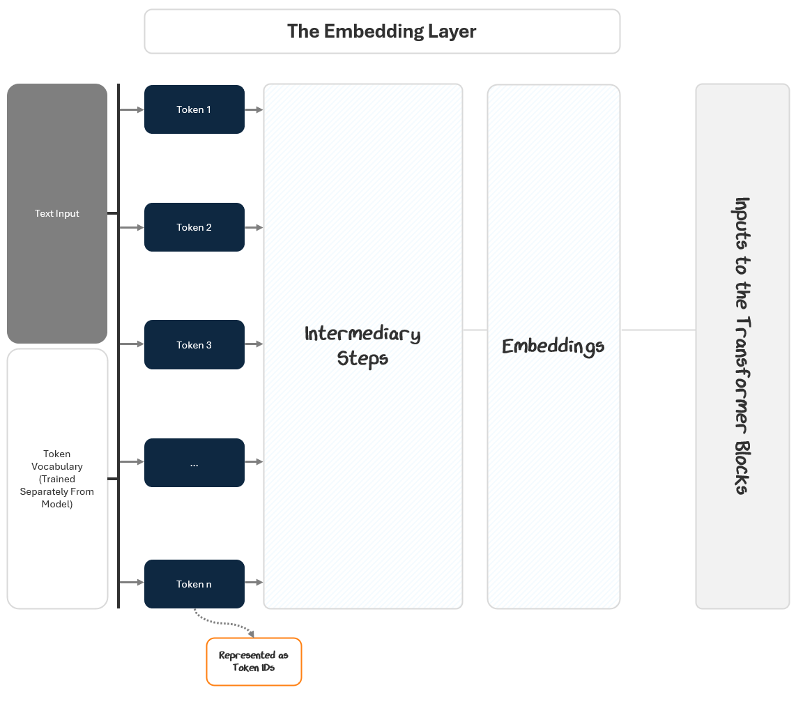
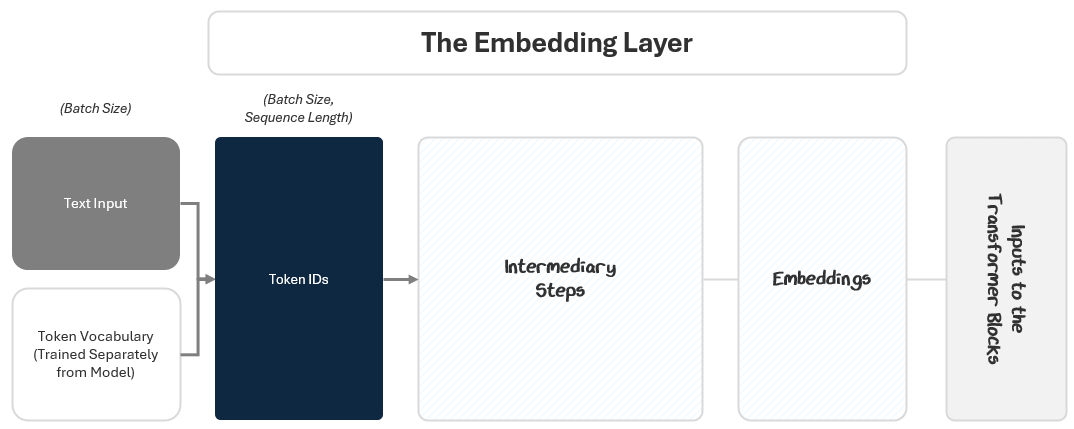
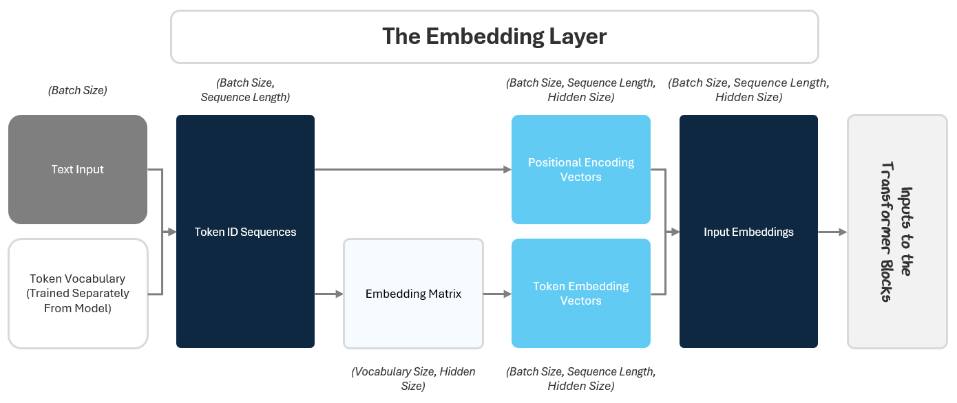
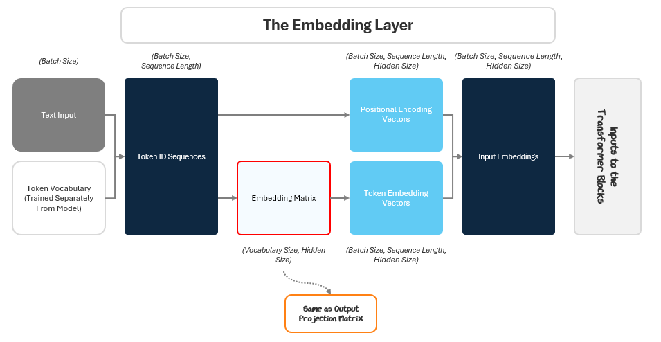
The Embedding Layer starts with the input text and outputs embeddings to the transformer blocks. It does this in two parts:

1. Turning the text into numbers

2. Turning the numbers into embeddings

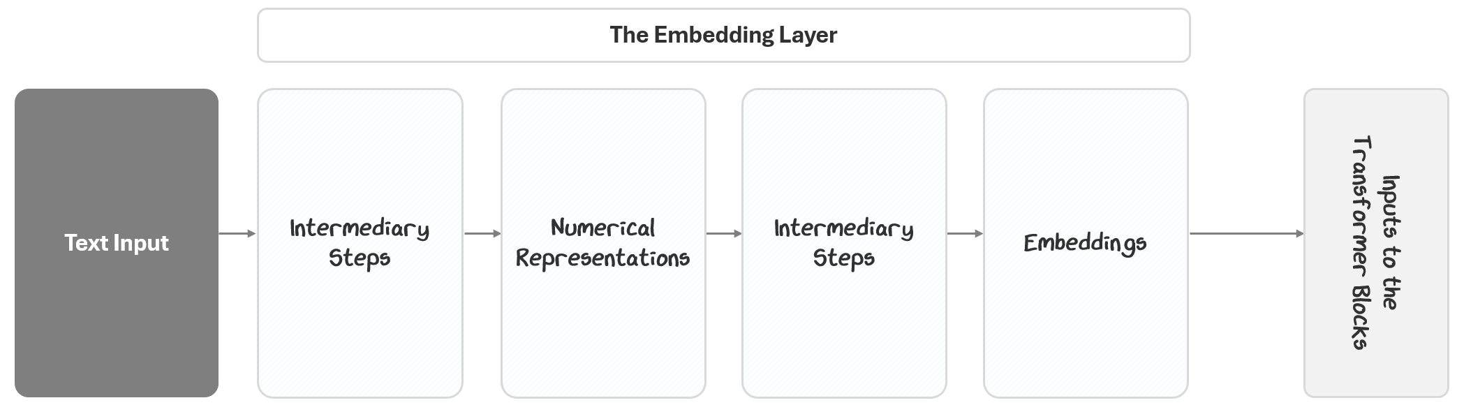
In this section, we’ll break out exactly how that happens.

1.1.1 Turning Raw Text into Useful Numbers via Tokenization

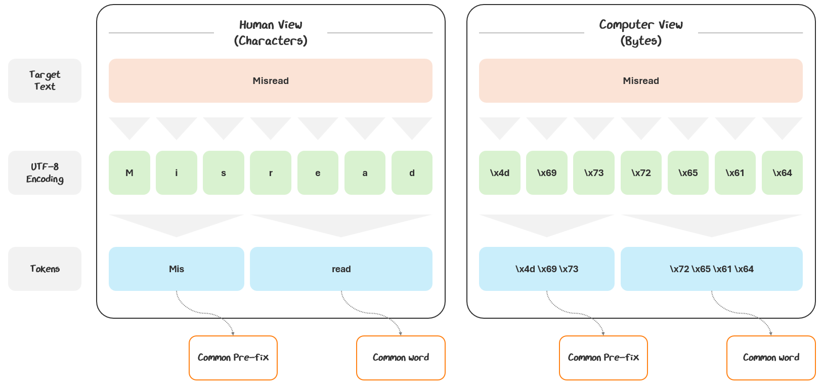
To turn the text into numbers, we use Unicode Transformation Format — 8-bit (UTF-8), a standard for encoding text into bytes. It’s a mapping system that turns every character into a numerical 1 to 4 bytes in length.

Source

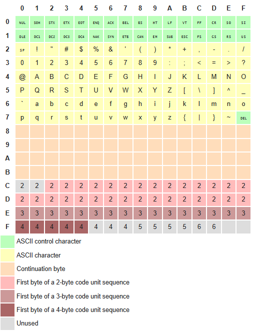
The power of UTF-8 is that it can cover millions of characters from languages and symbols around the world and seamlessly add new ones as they are invented.

• Simple characters (like English letters and numbers) use 1 byte — e.g., A = \x41 (the intersection of row 4 and column 1)

• More complex characters (like emojis, non-Latin scripts, or newly invented characters / symbol) use multiple bytes — e.g.:

  • é is two bytes (\xC3 the first byte of a 2-byte sequence and \xA9 a continuation byte. Together, they represent é.

  • 😂 is four bytes \xF0 \x9F \x98 \x82 — a 4-byte sequence indicator and continuation bytes.

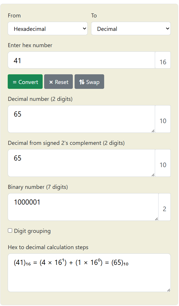
These bytes are the language that computers speak in and are effectively translated into a (binary) number for it to process. For example for “A” → \x41 (hexadecimal) = 65 (decimal) = 1000001 (binary).

Source

If you didn't understand this, don't worry. Just know that every character can be represented by a small number called a byte that computers can process.

However, if we fed those bytes directly into the model, we’d be giving it one tiny piece at a time — like trying to hand it a bread crumb and having it guess whether it came from a pizza or a sandwich. On their own, bytes are too small and too vague to carry meaningful patterns. For example, the word “hello” would show up as five separate bytes. That’s too low-level to capture meaning any sort of meaning.

So, we group UTF-8 bytes into tokens, meaningful chunks of characters that are commonly found together in language. A token isn’t necessarily a word. It might be a whole word, part of a word, or even punctuation. They are whatever units the tokenizer has learned are most useful for the model’s training.

The use of tokens helps models learn patterns in language efficiently, without departing from the flexibility to scale that comes from working at the basic byte level.

Words like “Misread” are great examples — tokenizers often break them down and reassemble the bytes into useful chunks like “Mis” and “read”, separating out the pre-fix.

So how do we go from text to tokens exactly? The process is called tokenization. Let’s see how it works.

1.1.1.1 Tokenization

To turn raw text into tokens, we use a tokenizer. The tokenizer takes raw text and chops it into tokens based on a pre-determined set of established tokens, called a vocabulary. The tokenizer looks at the text and maps each piece to one of the tokens in the vocabulary.

I know that’s a lot of jargon. Let’s walk through an example and turn the sample “Sorry, I misread.” into tokens, using an example vocabulary set.

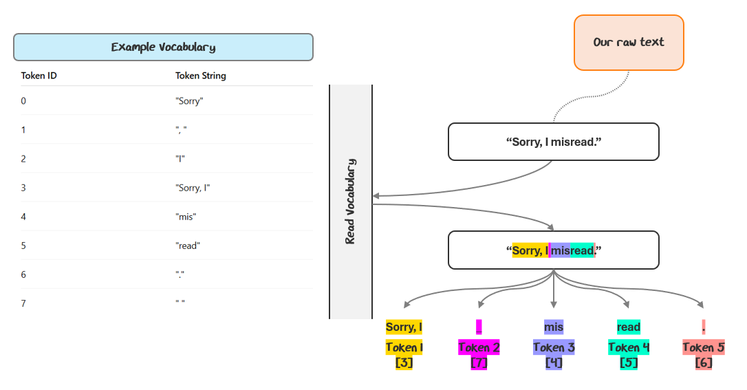
The tokenizer scans left to right, matching the longest possible tokens from a predefined vocabulary. So, “Sorry, I” is matched as one token, “ “ as another, “mis”, “read”, and finally “.” — each corresponding to a token ID.

The tokens are typically referenced to by their IDs in the vocabulary. So, the tokenization for this sequence would be [3, 7, 4, 5, 6].

Real-world vocabularies are much larger. OpenAI publicly shows their tokenizer, which supposedly contains 199k tokens in its vocabulary. Below, we can see how it maps inputs to the (behind the scenes) vocabulary.

Where does the vocabulary come from? It’s created independently from the GPT model. The model just queries the vocabulary, it doesn’t create it. If you’re curious how it gets made, check out the Appendix, Section 7.1 for a step-by-step walkthrough.

1.1.1.2 Structuring the Tokens in Data

The resulting picture is a parsing of the text input to tokens, using the vocabulary:

This is a nice visual diagram for us, but it doesn’t fully represent the full picture. First, it doesn’t show how computers are storing this information.

Computers store information in arrays. The number of dimensions there are to capture determines the shape of the array.

Source

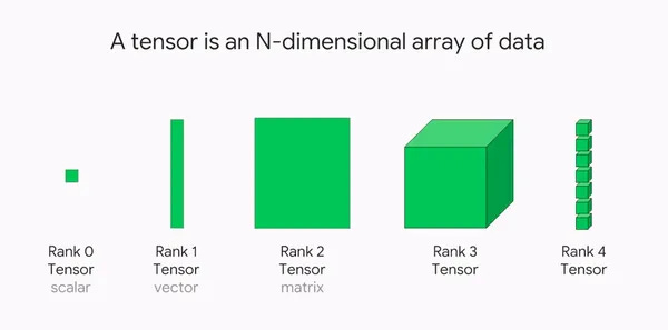
For example, a scalar is a single value or an atomic unit like a single string. When tokenizing, we are transforming that string into a sequence of tokens, which is stored in a vector.

To help keep track of data structure shapes, we describe the number of dimensions and the size of each through the following syntax:

We can use this to show that the Token IDs are a vector. The length of that vector is how many token IDs are in the sequence. So we represent the shape of the array with (Sequence Length).

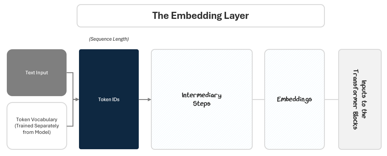
The second issue with our initial picture is that, it doesn’t capture that the text input we are ingesting is actually a vector of samples. Remember how we group samples together in “mini batches” from Part 1?

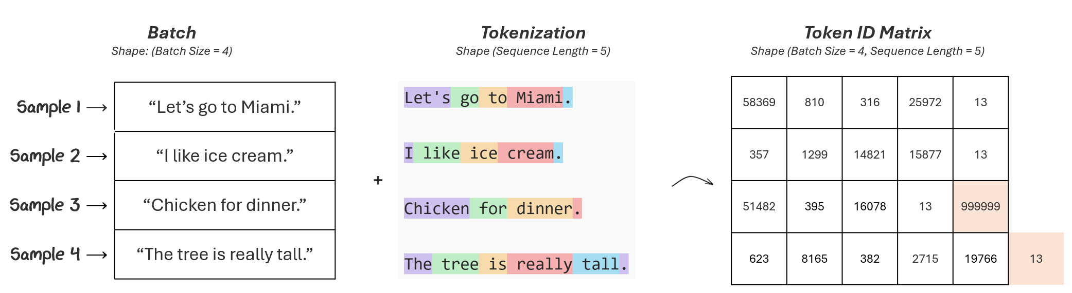
This mini batch has a size of 4 samples. It is of shape (batch size), indicating it is a vector (1-dimensional) and of length equal to how big the batches are (in this case 4 samples).

When tokenizing, we create a sequence of tokens for every sample separately. In our example, the token sequence is of shape (sequence length =5).

The shape of combined token matrix is (batch size, sequence length) — in this case 4x5.

You might notice that:

• “Chicken for dinner.” only has 4 tokens

• “The tree is really tall.” has 6 tokens

How do we create a common sequence length?

• To fix “Chicken for dinner.”, we add a padding token at the end to fill the remaining space

• To fix “The tree is really tall.”, we only keep the first 5 tokens. The last “.” is truncated off.

To make sure we aren’t wasting too much space or truncating too much data, we pick a sequence length that 90-95% of your samples can fit in. In this case, a sequence length of 5 seems to work well.

Incorporating the mini-batches of samples, we can update our visualization.

Our text input is a vector containing each of the samples in the mini-batch and our token IDs has a vector of token ID sequences for each mini-batch.

1.1.1.4 Recapping Tokens

We’ve now know how raw text makes its way into the model — not as words or letters, but as structured sequences of tokens.

• Text is stored as bytes using encodings like UTF-8. This is how computers represent language, but it’s too low-level and fragmented for a language model to learn useful patterns from.

• Tokenization bridges the gap by grouping bytes into meaningful, reusable chunks called tokens. Tokens are often whole words, subwords, or common patterns.

• These tokens are drawn from a predefined vocabulary, created statistically by identifying frequent character pairings in the training data. Each token has a unique token ID used by the model.

• Token IDs are organized into arrays, where each input sample becomes a row of token IDs in a matrix shaped like (batch size, sequence length).

• To align different-length sequences, we use padding (to fill short samples) and truncation (to shorten long ones), ensuring every input has a consistent shape.

The result is a 2D array of token IDs that can be turned into rich, contextual representations of meaning.

If you didn’t get all of that, don’t worry. It’s a lot. Here is the key idea: models don’t see words, they see token IDs, which are just chunks of text turned into numbers. These IDs are grouped into tidy arrays so the model can process them efficiently.

1.1.2 From Token IDs to Embeddings

We now have numerical tokens produced from our text, leveraging an external vocabulary. These token IDs insert content into the model, but it doesn’t know the definitions of these IDs. We now need to provide it with meaning and context.

To do this, we create two embeddings for each token ID:

1. A Token Embedding: This embedding gives each token a “starting meaning” based on how its generally used in language. For example, an embedding can indicate that the word “bank” could refer to both money or a river, like a comprehensive dictionary.

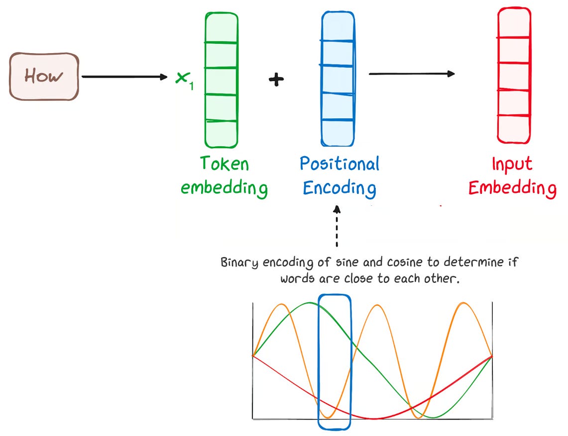
2. A Positional Encoding: This embedding tells the model where each token is in the sentence. This helps it know the order of the tokens, so it isn’t ingesting a nonsensical slop of words.

We then merge these two into a combined input embedding that captures everything we need to know about the token.

Let’s dive into how we create each embedding!

1.1.2.1 Token Embeddings

Just like how we used a token vocabulary to determine how to map our text to tokens and token IDs, we’ll use an embedding matrix to map a token to a token embedding. But, this time, the embedding matrix will be trained as part of the overall model — not separately like the vocabulary.

Here’s how it works:

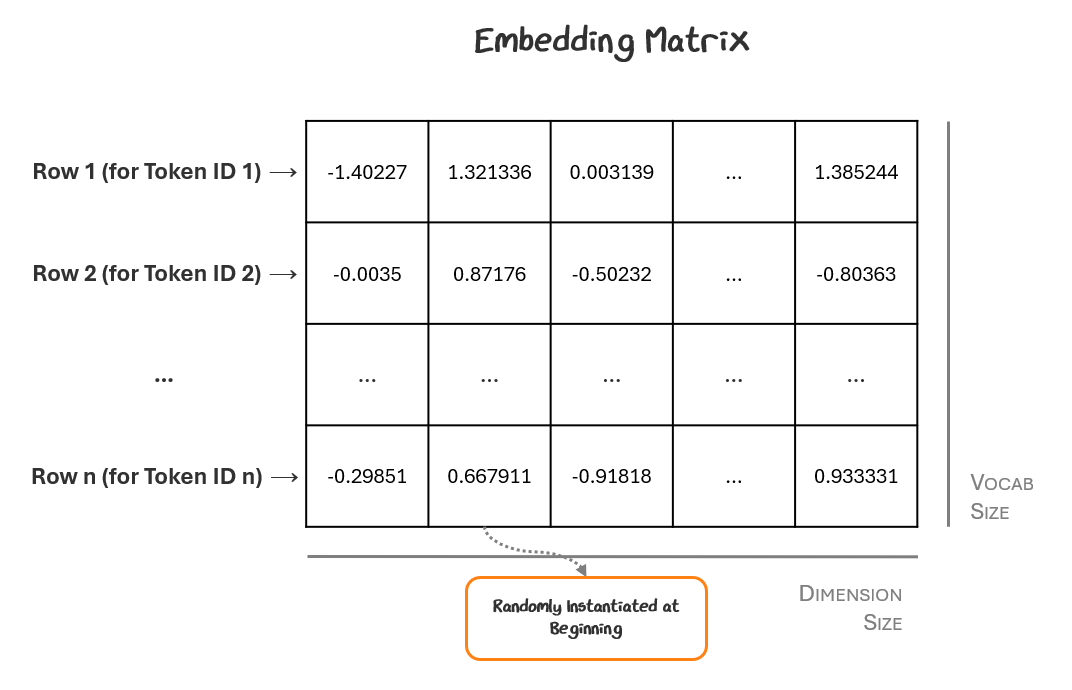
The embedding matrix is of shape (vocabulary size, embedding dimensions), so every possible token is listed, where embedding dimension is the length of the vector used to represent each token inside the model (e.g., 768 for GPT-2, 4096 for GPT-4o). This is also called the hidden size and is a design choice set by the model’s creators.

Every row in the matrix corresponds to a token ID and the values in that row represent the vector for that token embedding. To start, we put random values in each cell. It looks something like this:

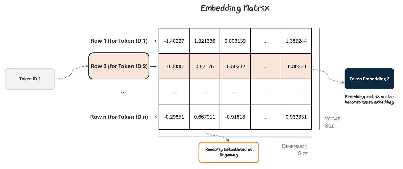
The model looks up each of its token IDs in the matrix to retrieve its vector, which is then used as the token embeddings for each token.

The embedding vectors aren’t hand-crafted. They’re learned during training just like any other parameter in the model. These token embeddings flow through the rest of the model, which generates an output, computes loss, and backpropagates gradients to update parameters. These gradients update the token embeddings and their corresponding slots in the embedding matrix.

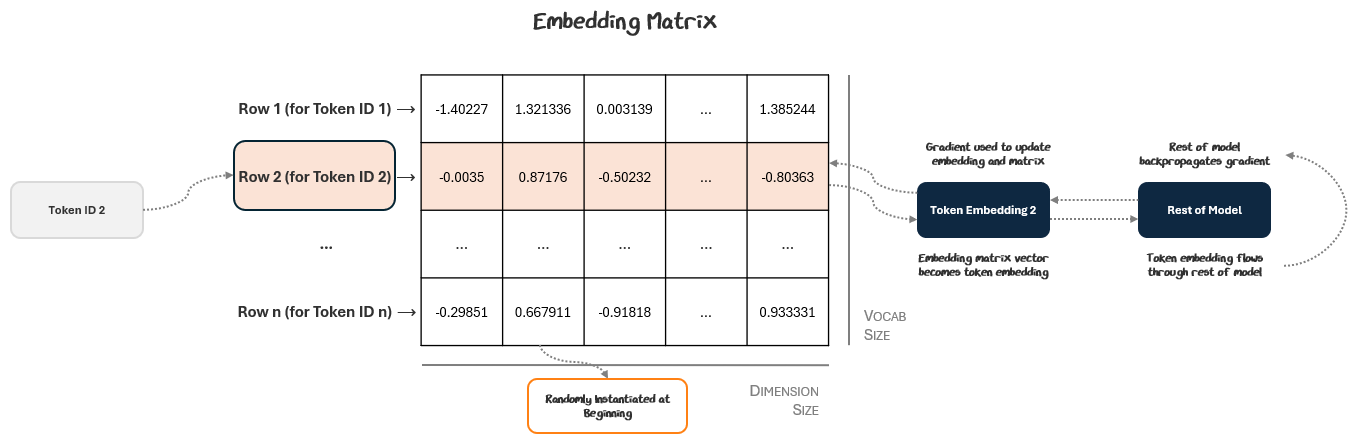
This process repeats and after enough training steps, the embedding matrix and its component token ID vectors become rich embeddings for the rest of the model to use. These embeddings contain learned semantics like how the word “bank” can be used both in the river and financial sense.

1.1.2.2 Positional Encodings

We now have meanings for the tokens, but model doesn’t know what the order is unless we explicitly give it to them. It needs to know where the words are in addition to their meaning.

The positional encoding is a technique for giving it this awareness. The positional encoding doesn’t simply keep track of “position 1, position 2, position 3” in a simple list. Instead, for each position (e.g., first token, second token), the model adds a unique vector that helps it track where each token is in the sequence.

To do this, we create a vector with alternating sine and cosine waves to encode position in the vector:

Adapted from here.

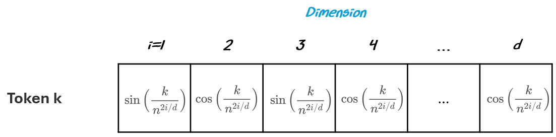
Where

• k is the position of the token in the sequence

• i is the index of the scalar in the vector

• d is the size of the vector (the hidden size)

• n is a researcher-defined scalar (e.g., 10,000 was used in the original Attention Is All You Need research paper)

Don’t worry too much about the specifics of the formulas. What’s important is that they are used to capture relative position and repeating patterns, described below.

The original models use sine and cosine because they capture:

• Relative Position: They make nearby positions have similar encodings and distant words have very different ones, helping the model know where and how far apart tokens are. With simply stating position 1, position 2, ... , the model doesn’t have the ability to subtract 3-1=2 to determine relative distance.

• Repeating Patterns: They create repeating patterns at different frequencies. This lets the model spot repeating structures — like the chorus of a song or a common phrase — even if they show up in totally different places.

• Richer Information: Using both sine and cosine together covers both the “rising” and “falling” sides of the wave, giving a richer representation. Sine and cosine are just shifted versions of each other (90 degrees apart), so having both helps the model pick up on different phases of the pattern. It’s like having both the longitude and latitude on a map.

Below is a vector filling with the positional encodings. We can kind of visually see how its encoding repeating patterns and relative positional context.

Source

But also, who knows… this is machine language now.

Sine and cosine waves were a good starting point, but newer models embed position in smarter ways, making them better at handling long or complex texts. We’ll revisit some of these new methods in Part 3.

1.1.2.3 Input Embedding

Each token embedding and positional encoding vector help the model know both what token it is seeing and where it appears in the sequence. Since it’s hard for the model to keep track of two distinct vectors for one token, we combine them into one.

To do this, we just add the two vectors together. The token embedding and positional encoding are vectors of the same size so they’re simply added together, element by element, before being passed into the model.

Source (Modified)

This might seem almost too simple, but it works: the model learns during training how to use this combined information effectively. Researchers have explored more complex ways of merging positional information, but this straightforward addition remains surprisingly effective for many tasks.

1.1.2.4 Recapping the Embedding Layer

The Embedding Layer transforms raw text into rich, model-ready input by stacking together four key steps:

• Tokenization: Break the text into meaningful chunks (tokens) based on a predefined vocabulary, giving the model pieces of language it can actually work with. There’s a sequence of tokens for every batch.

• Token Embedding: Map each token ID to a learned vector (of length hidden size) in the embedding matrix that captures its meaning. The vector is used as the token embedding and is refined over training as the model discovers patterns in language. There’s a token embedding for every Token ID in a sequence.

• Positional Encoding: Add information about where each token appears in the sequence, helping the model make sense of word order and relationships, using sine and cosine waves. There’s a positional encoding for every Token ID in a sequence.

• Combined Input Embedding: Add the two embeddings together to create the final input embedding for each token. There’s an input embedding for every Token ID in a sequence.

This combined embedding is the first thing the transformer “sees” — a packed summary of what the token is and where it fits. From here, the transformer blocks take over, refining these embeddings and building deeper understanding layer by layer.

Let’s go there next!

1.2 Transformer Blocks: Deep Processing

Now that we’ve transformed raw text into rich input embeddings, it’s time to transform them into new, more useful representations that can predict / generate the next token. While input embeddings capture the basic meaning and position of each token, they don’t yet capture how tokens relate to each other within a given specific sentence.

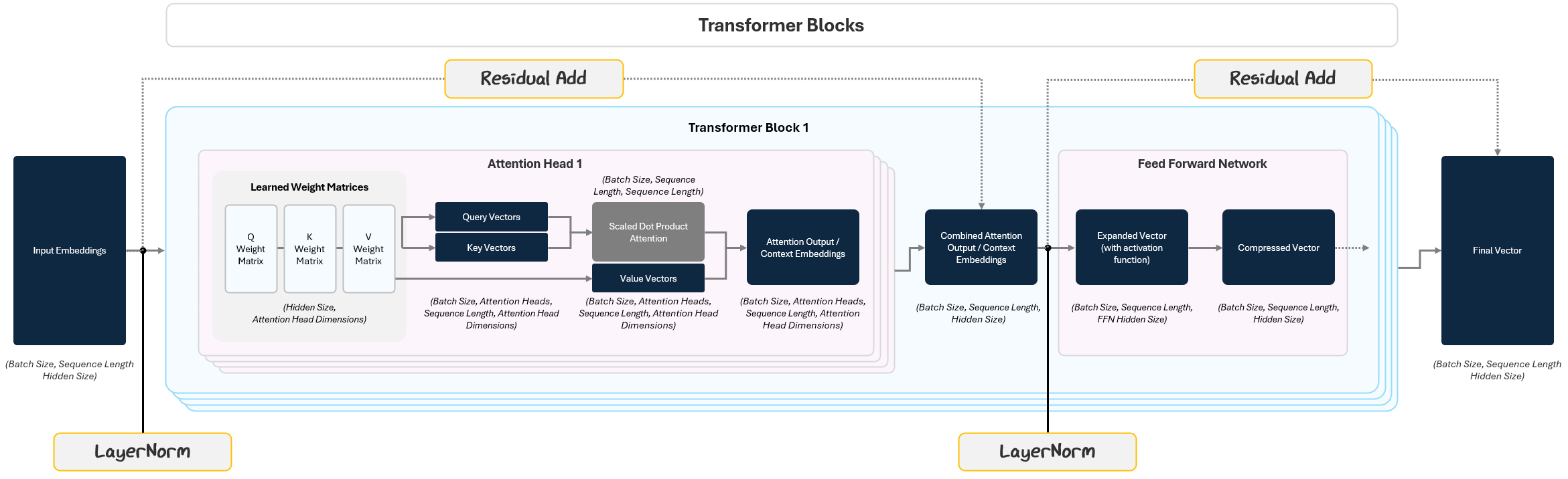
The transformer block is the heart of the GPT and was the breakthrough that spurred the massive rise of LLMs (more on this later). There are two parts to a transformer block:

• the Attention Mechanism

• the Feed Forward Network (FFN).

To help understand contextual meaning, Attention lets the model look at all tokens in the sequence and decide how they each individually relate to each other. It helps the model build a mental map of how words connect, highlighting the ones that matter most for making sense of the sentence.

After attending to other tokens, each token gets passed through a small neural network called a Feed Forward Network (FFN) that further transforms it, refining the meaning based on what it just learned in the attention.

This process repeats across multiple stacked transformer blocks (dozens or hundreds in big models) allowing the model to build up complex understanding from simple building blocks.

Let’s start with attention!

1.2.1 Attention

The key innovation behind the Transformer is self-attention. For each token, self-attention lets the model figure out which other tokens in the sequence matter, scoring how important each relationship is. Attention is like a weighted conversation between words. Some pairs of tokens will heavily influence each other while others will barely interact.

For example, if you’re processing the token “hungry” in “The cat that chased the mouse was very hungry”, attention helps the model realize it relates to “cat”, even though they’re separated by several words, and there isn’t much relationship with “the”.

Said differently, imagine you're at a loud cocktail party. Dozens of conversations are happening, but when you hear something that you can relate to, you tune in — you focus your attention on that conversation. In transformers, attention lets individual tokens "tune in" to the most relevant other tokens in a sequence when processing a given word.

Here’s how it works in practice.

1.2.1.1 Creating Attention Outputs

To represent how much each token attends (pays attention) to the other tokens, the model assigns a score for their relationship.

The model start this by applying three separate learned linear transformations to create the following for each token’s input embedding:

• Query (Q) Vector — What kind of relationships am I seeking with other tokens?

• Key (K) Vector — What kind of tokens should pay attention to me?

• Value (V) Vector— What information do I carry if you attend to me?

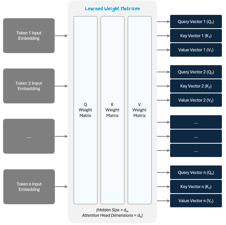
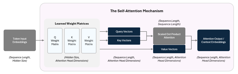
The Q, K, and V vectors are created by performing a linear transformation — i.e., multiplying the vector by a matrix.

• Our input, the input embedding, is a vector of size dₑ (embedding dimension / hidden size).

• We multiply it by a weight matrix of shape (dₑ, dₖ)

• The output (Q, K, V vectors) is a new vector of size dₖ.

So if your embedding is a 768-dimensional vector, and your model wants 64-dimensional Queries, your Query weight matrix would be (768 × 64). For example:

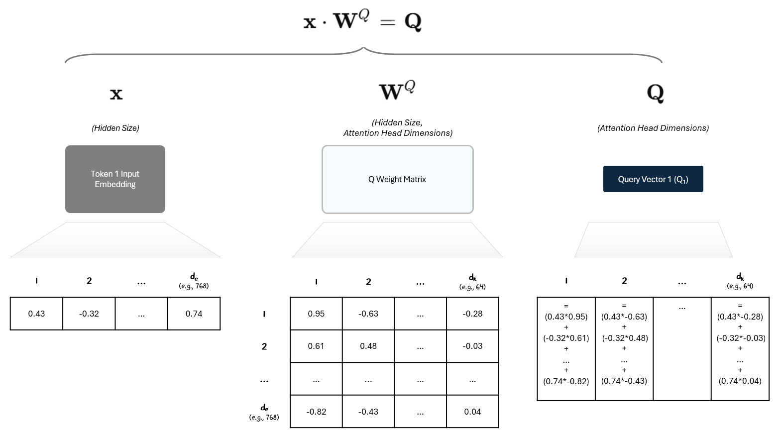
The three weight matrices (for Q, K, V) are shared across all tokens in a layer. They are initialized randomly and updated during training. Depending on how many dimensions the weight matrix has, the multiplication compresses or expands the input into a new space, just like a neural network does.

We then compare each query to all of the key queries to compute the attention score by performing a dot product on the two vectors.

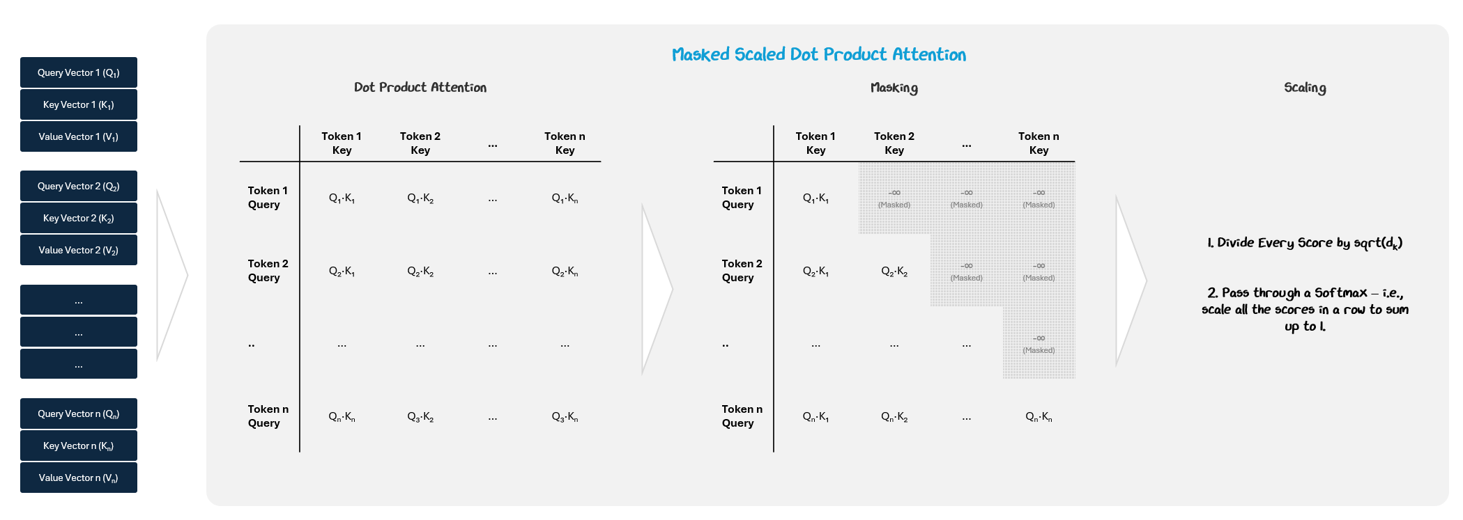
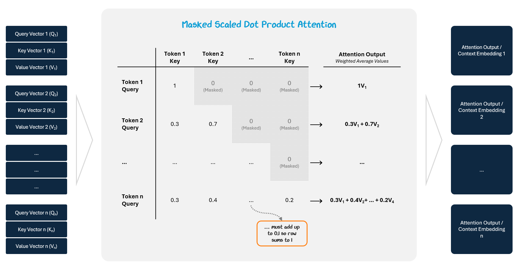
To prevent tokens from attending to future positions, a causal mask is applied to the attention score matrix. We make sure the model doesn’t “look ahead at tokens later on in the sequence by setting all values above the diagonal to negative infinity. This way, once we apply a Softmax, their value will become 0. This ensures the model generates outputs in a strictly left-to-right manner.

This gives an attention score showing how strongly the two tokens are connected. The scores are scaled (divided by √dₖ) to stabilize training and passed through a Softmax function (remember them from the Activation functions in Part 1?) to turn them into attention weights (they sum to 1).

Source

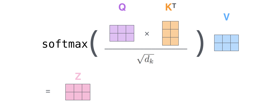
These weights are used to take a weighted average of the Value vectors, which are stored in an attention output (context embedding).

The result is a context-aware vector for each token that mixes in information from the tokens it attended to.

Putting our process together:

The model performs attention by updating the weights of the matrices that create the Q, K, and V vectors during training using backpropagation to reduce prediction errors. Over time, it learns to transform input tokens into Q, K, and V vectors that create useful attention patterns, like focusing on important words or relevant context.

1.2.1.2 Multi-Headed Attention

Rather than doing this process just once, the transformer block splits attention into multiple “heads”. Each head learns to focus on different patterns or relationships in the data in parallel.

Let’s go back to our cocktail party. Imagine you have multiple sets of ears, each tuned to pick up on different things. One listens for your name, a second listens for people who love your favorite TV show, a third for keywords related to your job, and a fourth that listens for mutual friends. Each ear focuses on a different signal in the noise, and together, they help you decide where to focus your attention and how to respond.

In the language model cocktail party:

• One head might focus on nearby words

• Another might focus on matching pronouns with their subjects or verbs with their subjects

• Another might connect a general statement to its specific examples (e.g., “fruits” to “apples, oranges”)

• etc.

Each head produces its own attention output (context vector) and after all heads finish, their outputs are:

• concatenated together

• passed through a final linear layer to merge them and bring them back down to the hidden size

resulting in the combined context embeddings. Below we can see how this splits out:

Source

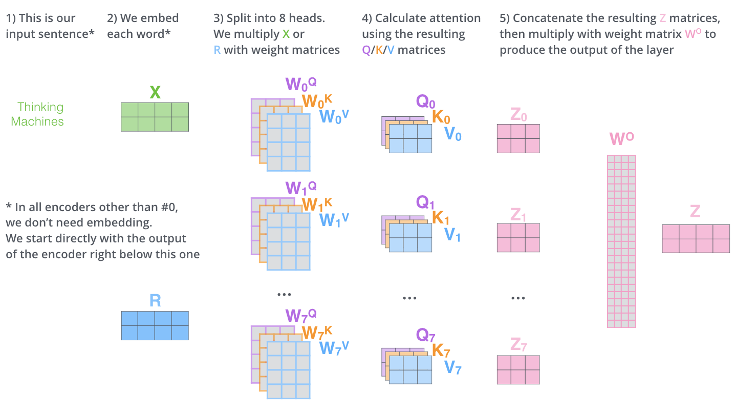
and summarized in our diagram format:

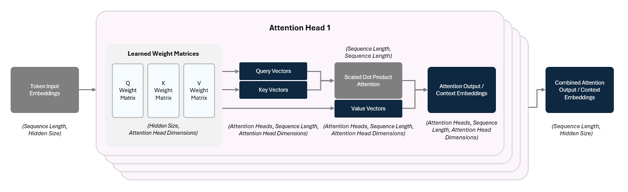
This is called multi-headed attention, and it lets the model capture different patterns in parallel.

1.2.1.3 Why This is an Important Breakthrough

Prior to the Transformer, LLMs (RNNs and LSTMs) were reading words one at a time and trying to carry that information forward step by step, which had two inefficiencies:

• Longer Term Relationships: The models had trouble capturing key relationships and patterns between words. They would forget older information or have difficulty learning patterns that depend on far-apart words.

  • For example: In the sentence, “The cat that chased the mouse was very hungry”, the model might lose track of “cat” by the time it reaches “was.” So if you asked it who was hungry, it might guess the mouse because its closer or wouldn’t even know.

• Sequential Processing: Instead of looking at all tokens in parallel like we are, RNNs / LSTMs processed tokens one at a time. Requiring a full pass of a model for every token is slow and inefficient.

Attention solved these two problems:

• it lets the model capture long-range relationships, even across paragraphs, by directly relating every token to every other token in the input.

• it allows the model to process all tokens in parallel, making training massively faster and more scalable.

This mechanism, repeated across multiple heads and stacked transformer blocks, gives GPT its ability to understand context, nuance, and meaning. In fact, many modern models scale attention massively. For example, GPT-3 uses 96 attention heads with 128 dimensions per head.

1.2.1.4 Updated Model

Let’s update our model diagram to incorporate Attention!

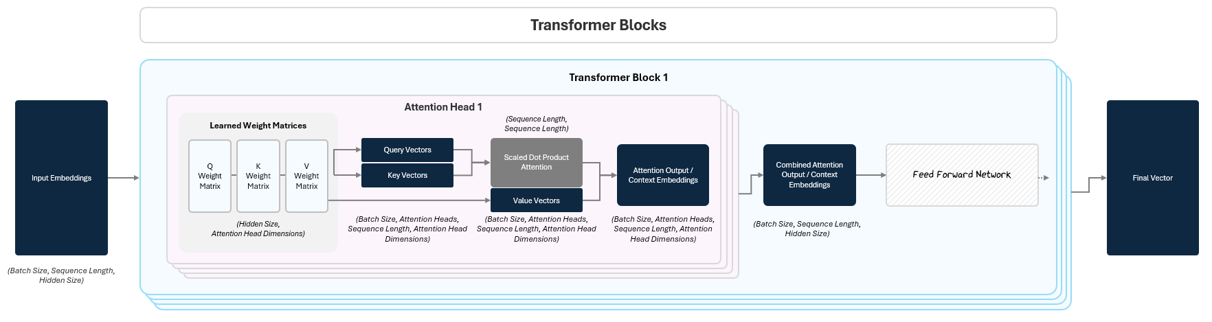
Now, let’s uncover Feed Forward Networks!

1.2.2 Feed Forward Networks

Once the attention mechanism lets each token gather information from others, the model still needs to process that information further. It does this through a Feed-Forward Network (FFN).

Think of attention as letting tokens have a conversation, and the FFN as each token reflecting on what it just heard. Attention mixes information between tokens and then the FFN processes each token in isolation.

1.2.2.1 How it Works

The FFN is a small, identical neural network applied to each token in the sequence, following this pattern:

1. Linear Transformation (Projection Up): The token’s vector is multiplied by a weight matrix that expands its size (e.g., by 4x). This lets the model move into a higher-dimensional space where it can express richer patterns.

2. Non-Linear Activation (e.g., SwiGLU) Function: The expanded vector passes through a non-linear activation function. This lets the model capture complex, non-linear relationships that a simple linear layer couldn’t.

3. Linear Transformation (Projection Down): The activated vector is then multiplied by another weight matrix that shrinks it back to its original size. This returns the token to the right shape for the next layer.

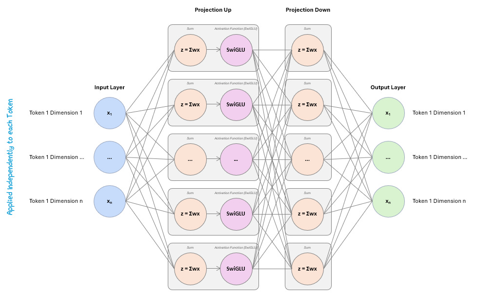
The output of this transformation is called the final vector.

1.2.2.2 Why This is Useful

The FFN gives the model two critical capabilities:

• Rich Non-Linear Transformations: It allows the model to learn non-linear patterns and transformations it couldn’t capture with attention alone.

• Depth and Flexibility: It refines each token’s representation before passing it to the next block, helping the model build more abstract and useful features over many layers.

Even though it looks simple, this two-layer FFN, repeated across dozens or hundreds of transformer blocks, is a key ingredient in the model’s ability to generalize.

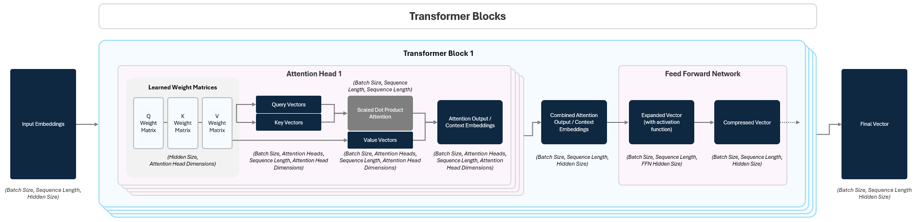
1.2.2.3 Updated Model

Let’s update our model diagram to incorporate the FFN!

1.2.3 Intermediary Steps to Improve Robustness

Attention and Feed-Forward Networks do the heavy lifting inside a transformer block, but without a few critical "maintenance steps," the model would struggle to learn efficiently.

This is where Layer Normalization and Residual Connections come in.

1.2.3.1 Layer Normalization: Keeping Activations Stable

As data flows through deep networks, the values of activations can easily drift —
getting too large, too small, or distributed inconsistently across layers.

Layer Normalization (LayerNorm) prevents this by standardizing the inputs of each layer so that each vector’s mean is 0 and variance is 1. This helps the model learn faster, avoid instability, and be less sensitive to initial random parameterizations.

This happens twice in every transformer block:

1. Before the Multi-Head Attention (on the input embeddings).

2. Before the Feed-Forward Network (on the output of the attention step).

1.2.3.2 Residual Connections: Don’t Forget Where You Started

Deep models are powerful because they transform data through many layers,
but this also makes it easy for information to get distorted or lost along the way.

Residual Connections solve this by passing the input of a layer straight to its output and adding them together. So instead of passing on only the transformed data, the model passes: Output = Layer Output + Original Input.

This simple addition does two important things:

• it preserves information from earlier layers

• it helps prevent a training issue where gradients get smaller and smaller the further back in the model

Residual connections are applied after both the Attention block and the Feed-Forward Network, making sure the original signal always stays in play.

1.2.4 The Full Transformer Block

In practice, models like GPT stack dozens or even hundreds of these blocks on top of each other. Each transformer block builds slightly richer, more abstract representations of the tokens. By stacking many blocks, the model can perform deeper processing — understanding everything from local syntax to global meaning.

The final output of the stacked transformer blocks is a set of deeply processed token vectors. These vectors now contain a rich, context-aware understanding of the input text. This is what gets passed into the next stage — the Language Model Head — which translates these representations into actual predictions, like the next word in a sentence.

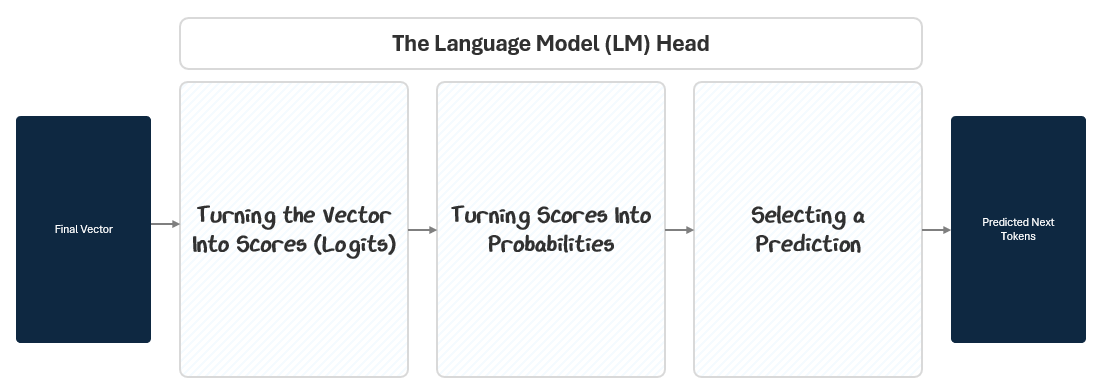
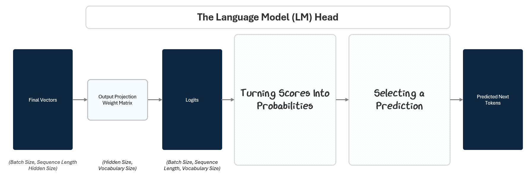
1.3 The LM Head: Turning Vectors into Token Predictions

By the time a token’s embedding passes through the transformer stack, it has been transformed into a deep, context-rich vector. But this vector is still abstract — it’s not a prediction yet. The Language Model Head (LM Head) converts this internal representation into a concrete output: the next token.

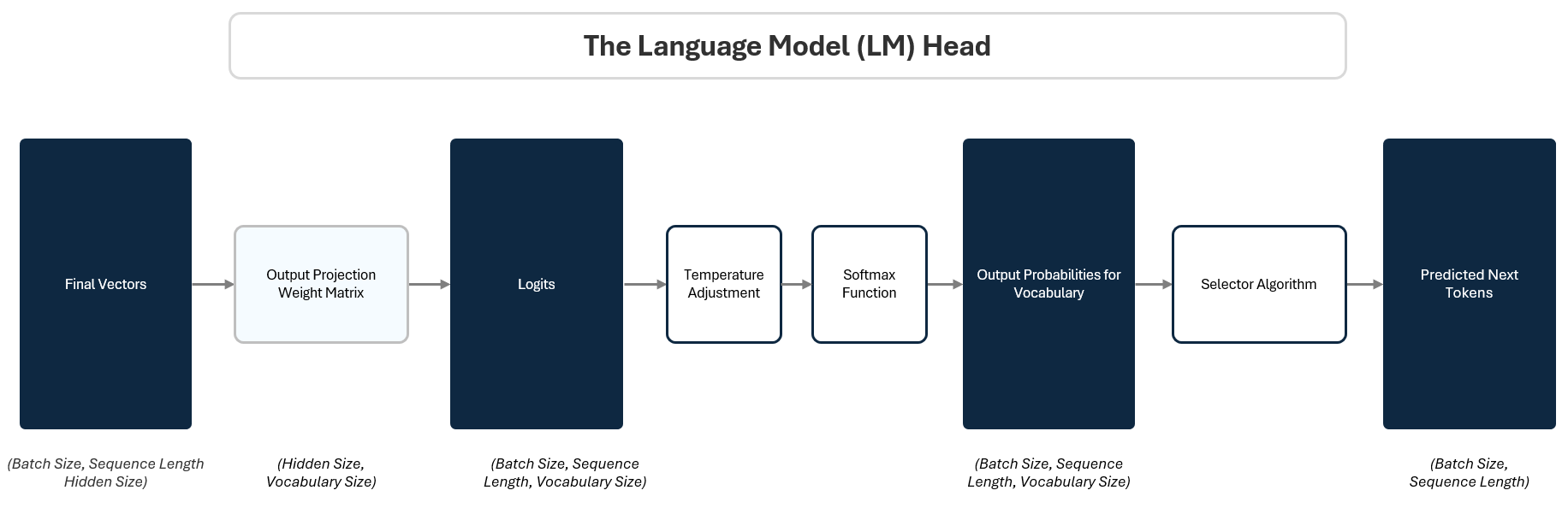
To do this, the LM Head passes the final vector through three steps:

1. Projection to Logits: A linear projection maps the vector to raw scores (logits) for every token in the vocabulary. This is like giving each possible token a stack of raffle tickets based on how likely the model thinks it should come next.

2. Softmax to Probabilities: A Softmax function converts those scores into probabilities. Based on how many raffle tickets each token in the vocabulary has, the model calculate a percentage probability of winning.

3. Selecting A Prediction: A selection algorithm picks the next token based on those probabilities. Like reaching into the raffle drum and pulling out a ticket at random. Tokens with more tickets have a higher chance, but every token with a ticket has a shot.

1.3.1 Projecting to Vocabulary Logits

The LM Head applies a simple linear transformation to the final vector of each token. This projection expands the vector from its hidden size to the size of the model’s vocabulary (e.g., 100,000 tokens). The output is called logits — raw, unnormalized scores for each token in the vocabulary.

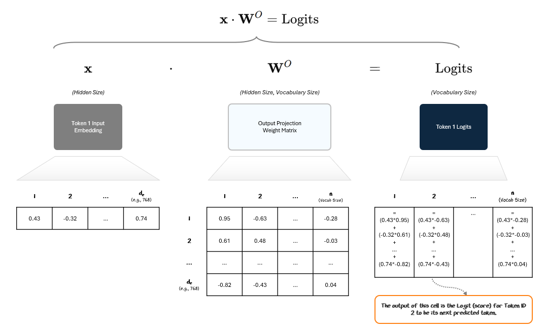
Each column in the Logits vector represents the score for that Token ID to be the next predicted token — i.e., how many raffle tickets that Token ID gets.

In most implementations, the LM Head’s output projection matrix is tied to the token embedding matrix from the Embedding Layer, meaning the matrices then share the same weights. This is called weight-tying.

Remember the Embedding Matrix from way back in the Embedding Layer? We reuse it as the Output Projection Matrix in the LM Head.

Tying the weights reduces the number of parameters and encourages consistency between how tokens are represented and predicted. We can think of it as encoding token IDs into embedding space at the input and using that same mapping in reverse at the output to decode from embedding space back into token scores over the vocabulary.

This gives us a set of logits, the model’s raw scores for each possible next token.

The next step is to turn these scores into probabilities.

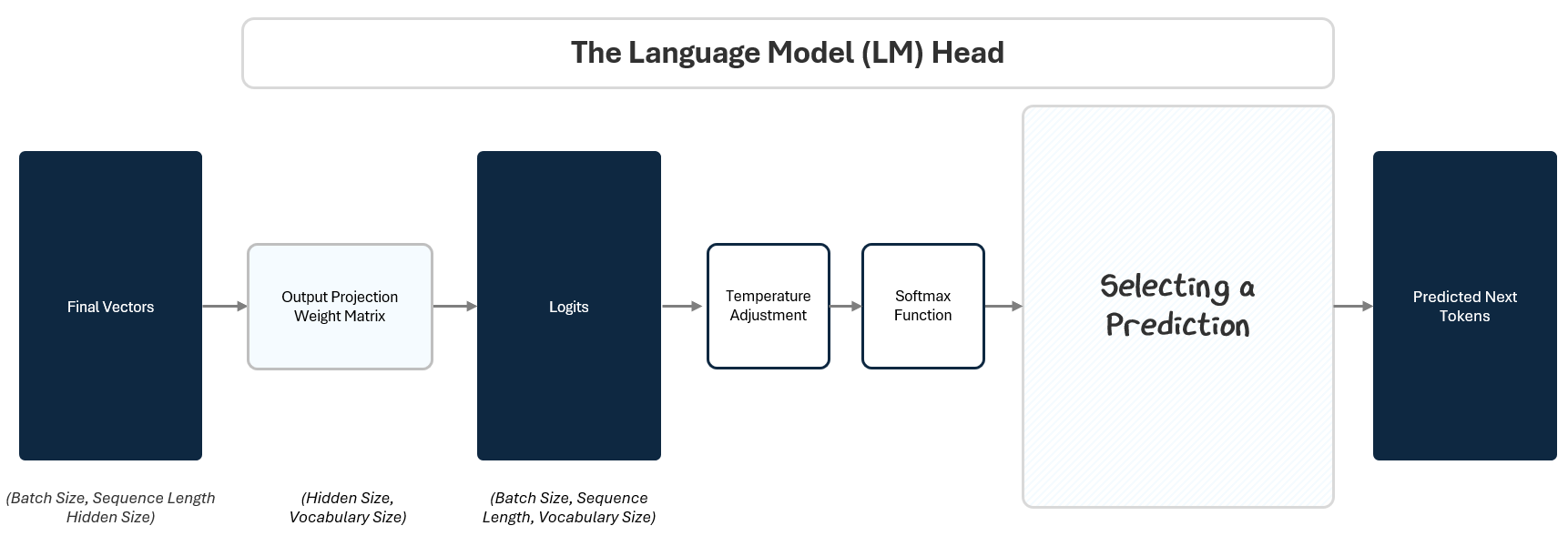
1.3.2 Turning Logits into Probabilities: The Softmax Layer

Logits themselves aren’t probabilities — they’re just raw scores. The model applies a Softmax function across the logits to convert them into a probability distribution. The Softmax function ensures two things:

• All values are between 0 and 1.

• The sum of probabilities across all tokens is exactly 1.

Higher logits correspond to higher probabilities after Softmax.

To incorporate more randomness, we can adjust the Temperature. Temperature is a single hyperparameter that controls how “confident” or “random” the model’s output is when we sample from its probability distribution.

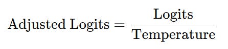
With temperature, we divide each logit by the Temperature before Softmax. Temperature acts like a dial for randomness — lower temperatures make the model more confident and deterministic; higher temperatures make it more exploratory.

Let’s say we are processing Token 1 “Hey” and trying to predict Token 2. We’ll project that Token 1’s final vector to logits using the output projection weight matrix and then apply temperature and Softmax to turn that into probabilities, ranking them from highest to lowest.

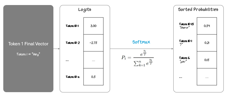
The next step is to use these probabilities to pick a next token.

1.3.3 Selecting the Next Token

Once we have a probability distribution over the vocabulary, the model selects the next token.

There are several algorithms to do this:

• Greedy Sampling: Pick the token with the highest probability.

  • In our “hey” example, we would select “there”

• Top-k Sampling: Pick randomly among the top k tokens.

  • In our “hey” example, if we select k=2, we would have a 50/50 pick between “there” and “!”.

• Nucleus (Top-p) Sampling: Pick randomly from the smallest set of tokens whose combined probability exceeds p.

  • In our “hey” example, if we select p = 0.9, we pick randomly from “there,” “!” and “you”, the smallest set of tokens whose combined probabilities add up to 0.9.

These sampling methods control whether the model plays it safe or takes creative risks. Top-p sampling, with temperature, is most common today to give controlled randomness to output.

And now we have our predicted next tokens!

These three steps — projecting, normalizing, and sampling — are the final bridge between the model’s internal reasoning and the words we actually see.

1.4 The Big Picture (Literally)

We’ve now completed our diagram for the GPT architecture!

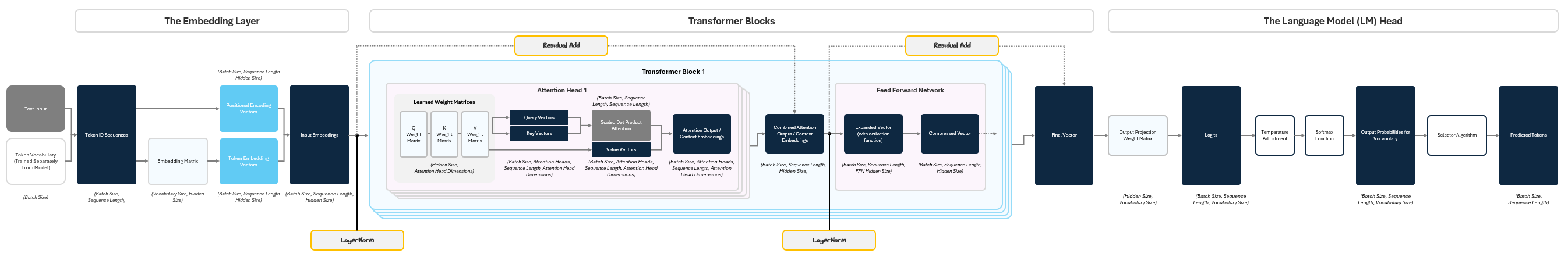
Pat yourself on the back, that was a long journey.

We’ve walked through each piece of the transformer blocks — from turning raw text into token embeddings, to passing those embeddings through attention layers, feedforward networks, normalization, and finally projecting them into token predictions. Each step might seem straightforward on its own, but stacked together, they create remarkable power.

The Transformer’s core innovation lies in how it lets each token attend to every other token, processes them deeply with multiple layers, and learns to transform these representations over and over again. This simple, modular design scales incredibly well, allowing models to learn everything from basic grammar to reasoning, coding, and creative writing.

1.4.1 Complementary Visualizations

If you want to see this all visually, there are fantastic interactive tools online that bring the architecture to life.

The Transformer Explained Visually (poloclub.github.io) lets you step through examples to see how the data flows through the architecture.

LLM Visualizer (bbycroft.net) gives a modular overview of the entire architecture and how components flow together.

Seeing how the model processes an input can help solidify your understanding data flows and relationships. Play around with them!

1.4.2 Adding Depth to this Architecture

Several key design choices shape the capability of a Transformer model:

• Depth: How many transformer blocks are stacked on top of each other.

• Width: The size of the hidden vectors inside each block.

• Attention Heads & Head Size: How many attention heads each block uses, and the dimensionality of each head.

• Context Window: How many tokens the model can attend to at once.

Together, these control how much information the model can capture, hold, and process in context. All of this is broadly summarized by a model’s parameter count — the total number of learned weights across the entire network. These parameters are what the model tunes via backpropagation during training. The bigger the model, the more capacity it has to learn complex patterns, though with that also comes bigger computational costs.

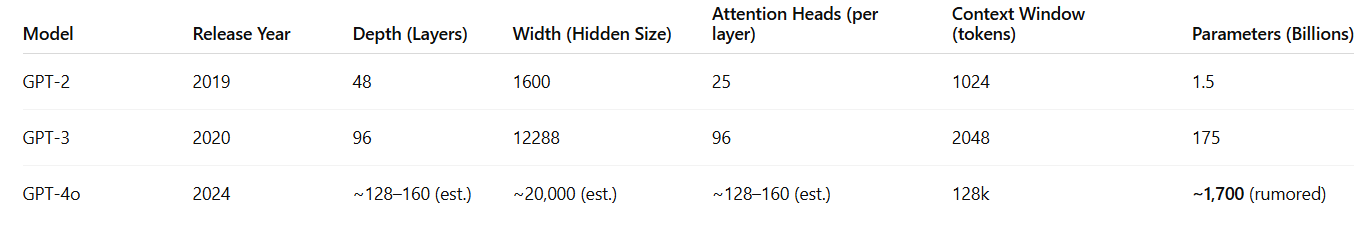
In modern models, parameter count has entered into the trillions and is only expanding.

Now that we’ve built the architecture, let’s see how training turns this into a working chatbot.

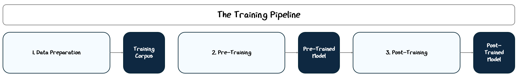
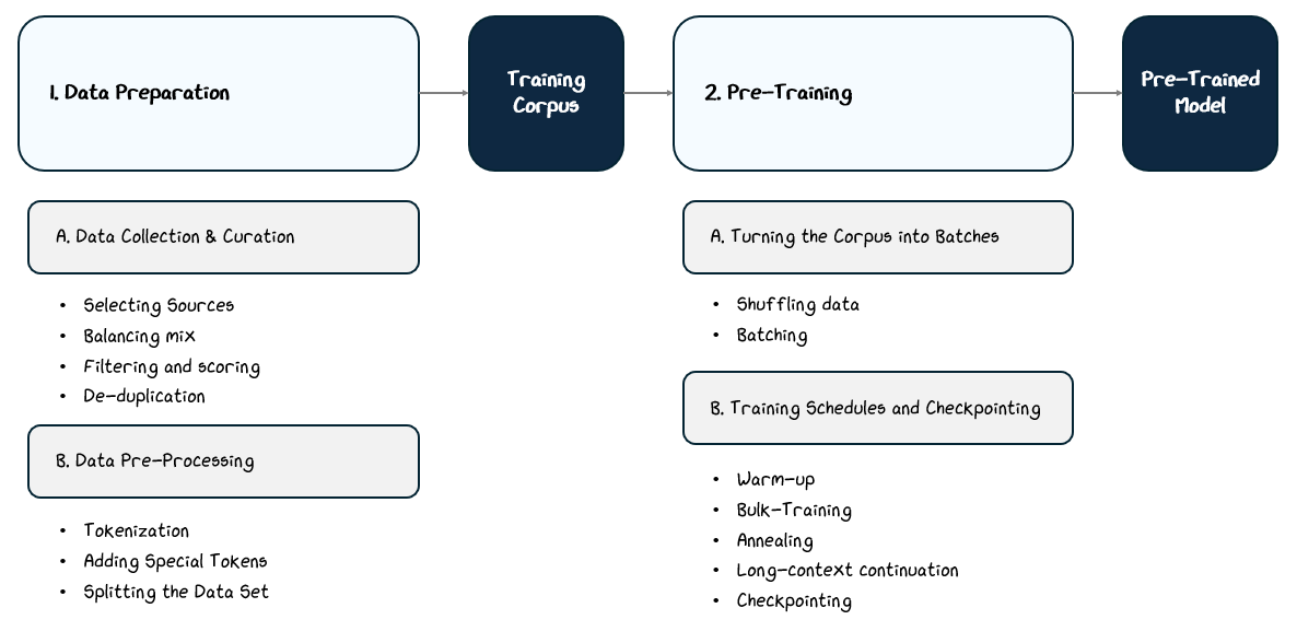
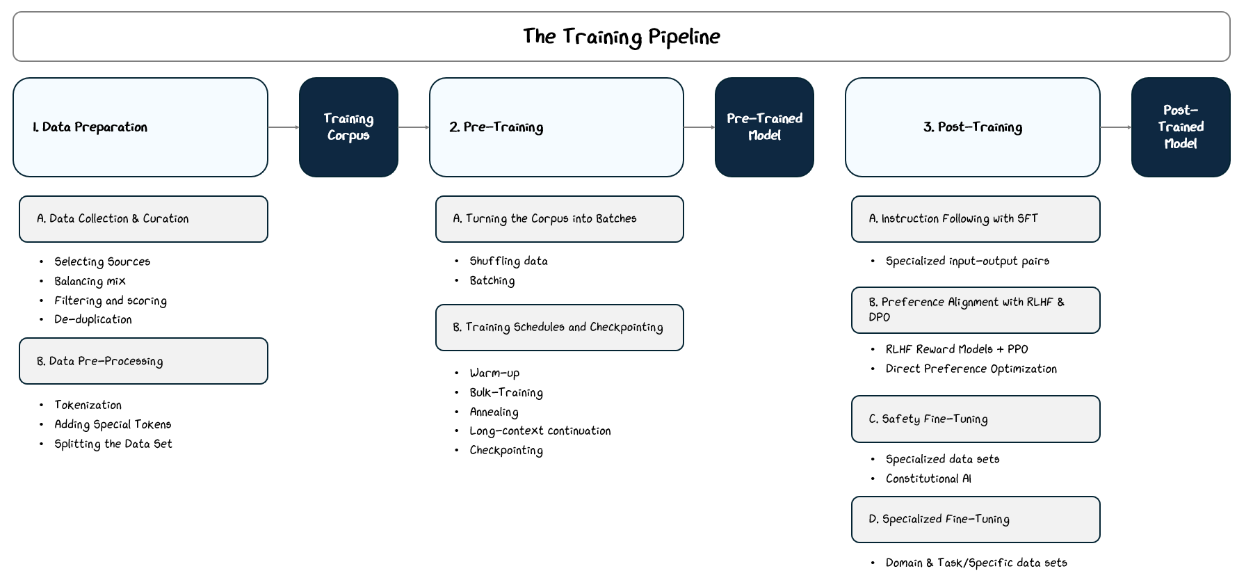
2. Training: From An Architecture to a Full Chatbot

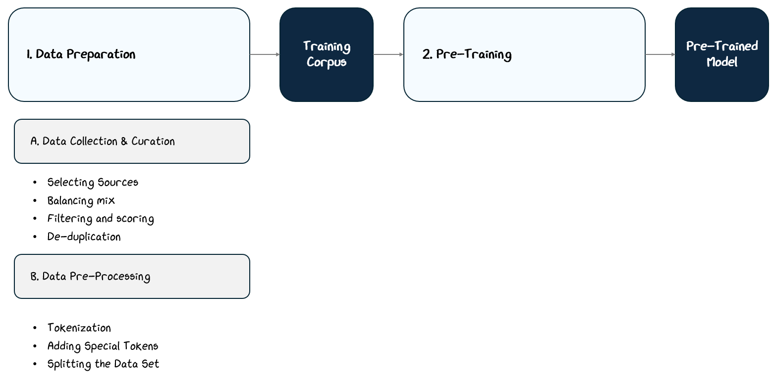
We’ve built the model, which is basically a big stack of math layers, but it’s useless until we train it. The training process happens in three main broad steps:

1. Data Preparation: Collect over a trillions of tokens from books, websites, and other public sources, and clean and process it to create the training corpus.

2. Pre-Training: Train on this corpus with a next-token prediction as the learning objective.

3. Post-Training (a.k.a Fine-Tuning): Further train the model on curated datasets with specific goals, such as instruction following, dialogue, or alignment with human values.

Let’s get into Data Preparation.

2.1 Data Preparation: Creating the Corpus of Text

Large language models depend on vast amounts of text — far beyond what any human could read in a lifetime. Collecting text is only the starting point, as the data must also be curated, processed, and shaped into a form the model can learn from most effectively.

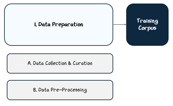
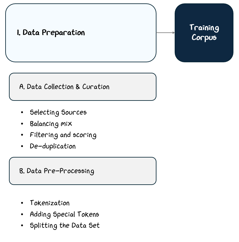
This preparation process typically unfolds in three stages:

1. Data Collection & Curation: Gathering diverse sources, balancing content types, filtering for quality, and removing duplicates.

2. Data Pre-processing: Converting raw text into a structured format the model can use, including tokenization, special tokens, and splitting datasets.

Together, these steps transform raw, messy text from the internet into a refined training corpus, laying the foundation for the model’s learning process.

2.1.1 Data Collection & Curation

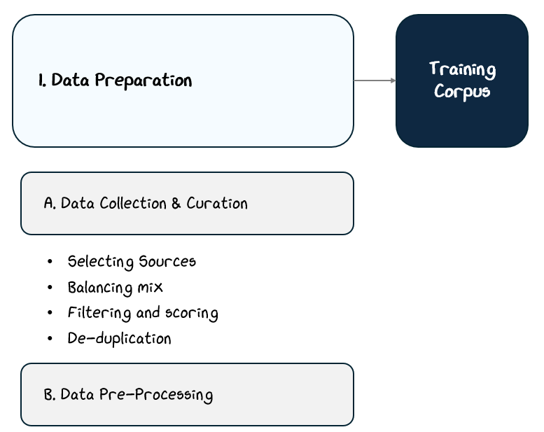
Data collection and curation typically follow four key steps:

1. Selecting diverse data sources and collecting data

2. Balancing the mix of content types

3. Filtering and scoring for quality

4. Removing duplicates or redundant content

Each step helps ensure the final training corpus is broad, representative, and suitable for training a general-purpose language model.

2.1.1.1 Selecting Sources and Collecting Data

The first step in preparing training data is deciding where to collect it from. Since large language models rely on exposure to a broad range of language styles, topics, and domains, the dataset needs to reflect this diversity. Researchers start by identifying key source types, including books, websites, academic papers, news articles, and open-source code repositories. The aim is to capture both formal and informal language, technical writing, creative fiction, conversational dialogue, and more to give the model a wide foundation to learn from.

Data is typically gathered in several ways:

• Public Downloads: Open datasets, public domain books, and open-access research archives are often downloaded directly.

• Web Crawlers: Automated tools scrape publicly available web pages (e.g., CommonCrawl), sometimes filtered by domain lists or quality signals to avoid low-value content.

• Open Code Repositories: Code examples are collected from platforms like GitHub, within licensing limits, to expose the model to programming languages and technical formats.

• Proprietary or Licensed Data: Some organizations may purchase and incorporate proprietary datasets to complement public data sources. These can include licensed book collections, commercial dialogue transcripts, subscription-based news archives, or curated datasets acquired from publishers or data vendors.

• Synthetic Data: In some cases, researchers introduce machine-generated text produced by earlier models or algorithmically. Synthetic data is primarily used to address gaps or deficiencies in the natural corpus by introducing rare language patterns, structured formats, or edge cases.

Putting this together results in a widely varying corpus. For example, we can see how The Pile, a massive, diverse open-source text dataset created in 2020–2021 pulls from a wide variety of sources like PubMed and FreeLaw to Wikipedia to build its data set.

Source

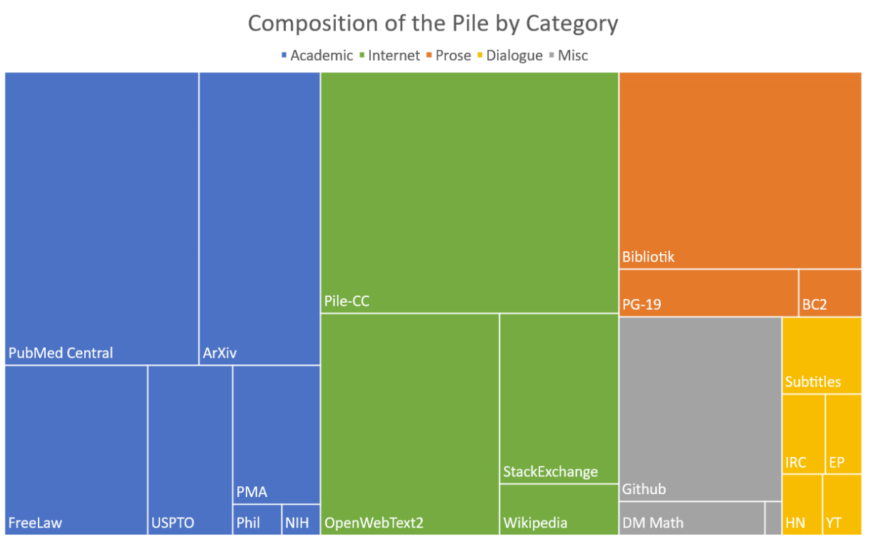
In addition to the sources, researchers also consider metadata such as publication date, source reputation, or author credibility. These factors help ensure the data is relevant, high-quality, and representative of current language use.

Ultimately, researchers are looking for sources to help the model learn language, generalized across tasks, domains, and language styles and will shape the corpus accordingly. We all want to be well-versed right? Why not a model too! We’re building a reading list for the most curious student on Earth — one who wants to learn law, write poetry, translate code, and answer trivia all at once.

2.1.1.2 Balancing the Mix

After collecting data from diverse sources, the next step is balancing the mix of content types. Without careful balancing, a dataset might end up dominated by certain domains — e.g., if there are too many fiction books in the corpus, then the model might be really good at making up a creative story, but not as good as answering a question with facts.

To avoid this, researchers define target proportions for each domain based on the model’s intended use cases. They may allocate specific percentages to fiction, nonfiction, conversational text, technical documents, or code.

Once the target mix is set, researchers adjust how much data they take from each source. They might take extra from some sources to make sure they’re well represented, or take less from others to avoid having too much of one type.

Balancing isn’t a one-time task. Researchers often monitor and refine the mix based on exploratory analysis or results from early training runs. If a model shows unexpected biases or weaknesses in certain domains, adjustments may be made to the dataset composition before final training begins.

2.1.1.3 Scoring and Filtering for Quality

Once data has been collected and balanced, it still needs to be checked for quality. Not every piece of text is useful for training a language model. Some may be poorly written, incoherent, nonsensical, offensive, or irrelevant. We’ve all seen some of the quality of content on the internet — we certainly don’t want all of it informing what is supposed to be a highly intelligent model.

Filtering and scoring help remove this unwanted material before it reaches the training phase. The first layer of filtering typically relies on automated heuristics — simple rules designed to catch obvious issues. These can include checks for language detection (to remove non-target languages), grammar or formatting errors, excessively short or repetitive content, or broken markup. This helps eliminate obvious noise, spammy content, or malformed data.

Beyond heuristics, some pipelines use statistical or algorithm-based scoring systems. These systems might be trained (separately from the model) on labeled examples of “good” and “bad” text, allowing them to assign quality scores based on factors like coherence, readability, or originality. For example, a scoring model might flag text that looks like low-effort spam, gibberish, or toxic language and highlight really well written articles.

Filtering and scoring are critical because the quality of the training data directly impacts how well the model learns. It affects not just its performance, but also its reliability, safety, and potential for harmful behavior.

2.1.1.4 Removing Duplicate or Redundant Content

After filtering and scoring, the dataset still needs to be checked for duplicates and redundant content. Large-scale text datasets often contain repeated material, whether it’s the same article published across multiple websites, boilerplate text reused within documents, or common phrases and templates. If left unchecked, this repetition can distort training by giving certain examples undue influence or causing the model to memorize content instead of generalizing from it.

Deduplication isn’t just applied within a single dataset but also across datasets when multiple sources are combined. Two passes through the data are made

1. First, exact duplicates (identical strings of text) are removed using hashing algorithms or simple text matching. This ensures that identical documents or paragraphs aren’t fed to the model multiple times.

2. Second, near-duplicate detection is applied to catch cases where the wording is slightly different but the content is effectively the same — for example, syndicated news articles with minor edits. This often involves using similarity metrics or embeddings to flag and remove overlapping content.

With sources selected, content balanced, quality filtered, and duplicates removed, the collected data is finally shaped into a broad, representative corpus. It’s ready for the next critical step: turning it into a format that a machine can process.

2.1.2 Data Pre-processing

Once the data has been collected, curated, and cleaned, it still isn’t ready for training. Large language models can’t process raw text, they work with tokens. Data pre-processing handles this before training so that the model doesn't waste time or compute power handling raw text during training runs.

This stage typically includes four key steps:

• Tokenization: Converting raw text into sequences of tokens.

• Adding Special Tokens: Inserting control markers that help the model understand context, tasks, or conversation boundaries.

• Splitting the Dataset: Dividing the data into training, validation, and optional test sets to ensure proper evaluation and avoid overfitting.

Together, these steps ensure that the dataset is both structured for the model’s architecture and optimized for scalable training.

2.1.2.1 Tokenization

The first step in pre-processing is tokenization: converting raw text into discrete tokens and assigning each token a unique numerical ID from a fixed vocabulary. We covered this process all the way back in 1.1.1.1 with Tokenization and in the Appendix Section 7.2 with Byte-Level Byte Pair Encoding.

The output of this process — a long sequence of token IDs — forms the basis for all further processing and training.

2.1.2.2 Adding Special Tokens

During or after tokenizing raw text, special tokens are inserted to give structure or provide signals that guide the model’s behavior. These tokens serve functional purposes that are critical for training and inference. Common examples include:

• Beginning/End-of-text markers that signal the boundary of a document or conversation (e.g., <|begin_of_text|> and <|endoftext|>).

• Instruction or prompt tokens that differentiate between roles or segments in a dialogue (e.g., <|user|>, <|assistant|>).

• System or control tokens that convey metadata, task cues, or formatting guidance.

Special tokens act as signposts within the token sequence, subtly steering the model’s and its outputs as it learns structural patterns. This improves the model’s ability to handle a broad variety of contexts like creating documents, multi-turn dialogue, follow instructions, and generalizing across different tasks.

2.1.2.3 Splitting the Dataset

Once the data has been tokenized and prepared, it is divided into distinct subsets to serve different roles in the training process.

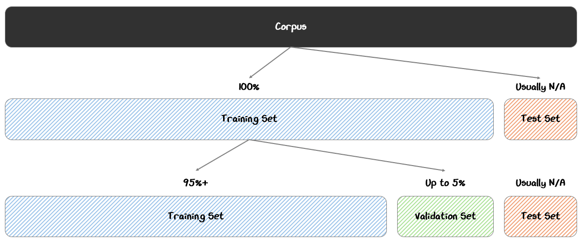
The most common split includes:

• Training Set (95%+): The bulk of the data, used directly to update the model’s weights during training.

• Validation Set (Up to 5%): A separate portion of data held out from training, used to monitor the model’s performance and tune hyperparameters during training

• Test Set (Optional): An additional reserved set, used after training to assess the model’s final performance on truly unseen data

The training set is like the study guide, the validation set is like the practice problems, and the test set is like the actual exam.

The model learns better when exposed to as much data as possible, so using 95%+ for training ensures the model sees the broadest range of language patterns while still leaving enough validation data to monitor overfitting and guide training decisions like early stopping or learning rate adjustments.

In typical machine learning, we often reserve a test set as a final holdout to evaluate the model after training. However with LLMs, the validation set is sufficient, since separate evaluation tools are used after training to assess more complex tasks than just next-token prediction.

2.1.3 Recapping the Training Corpus

With the data collected, curated, filtered, and tokenized, the final corpus represents the foundation on which the model will learn. The quality and composition of this corpus directly influence how well the model learns patterns, generalizes across tasks, and performs in real-world applications.

This requires thoughtful collection and curation of the data set, which is then turned into digestible pieces for the model. With the corpus prepared, the next step is to put it to work, feeding it into the model during pre-training to begin the process of learning from data.

2.2 Pre-Training

Pre-training is where the model begins to learn, turning the massive, carefully prepared corpus into patterns it can internalize. As with the neural networks from Part 1, the model processes sequences of tokens, makes predictions, computes loss, backpropagates gradients to update its weights, repeating this cycle until the loss decreases.

Three key ingredients make large-scale pre-training possible:

• The Transformer architecture allows the model to predict the next token at every position in parallel, a design that makes training far more efficient.

• The massive corpus is split into batches of token sequences, which are processed in parallel across distributed systems.

• Training follows carefully designed schedules, which tune learning rates and the data the model is fed for optimal results

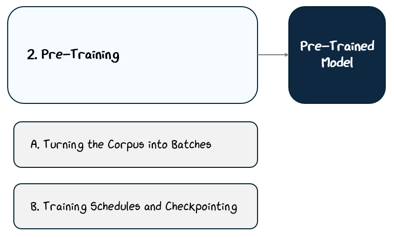
Together, these elements turn the static corpus into a dynamic learning process, scaling up from individual token predictions to massive, distributed training that powers modern language models.

2.2.1 How Architecture Enables Efficient Training

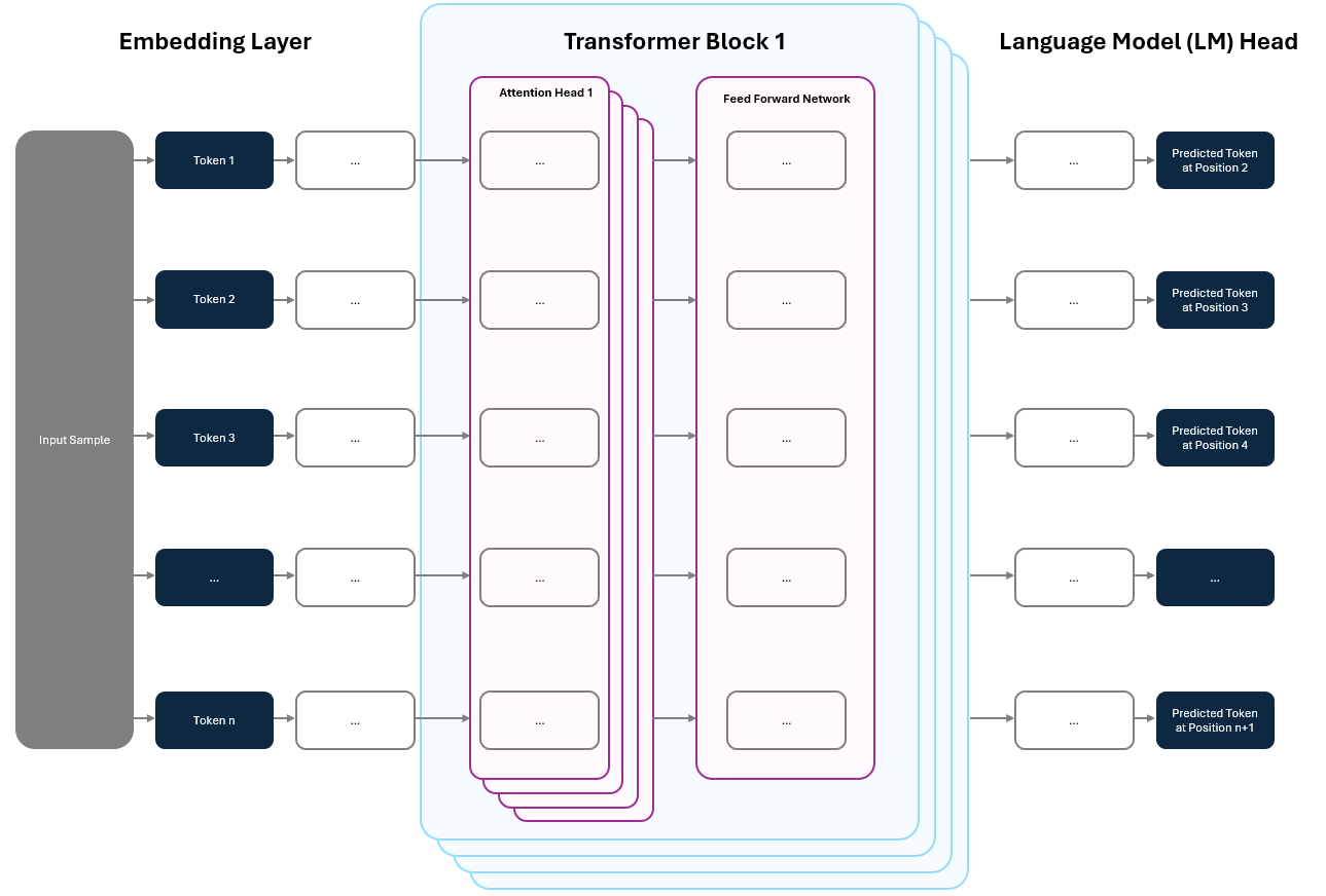
One of the most powerful features of the Transformer architecture is how naturally it lends itself to efficient training. When the model ingests data, it doesn’t just predict the next token for a single position. It predicts the next token at every position in the sequence, all at once.

In a contracted diagram from Section 1, this appears as “Predicted Next Tokens”, which has the shape (Batch Size, Sequence Length), meaning the model makes a prediction for every token position across all samples in the batch.

Zooming into a single sample in a single batch, we can see the predictions at every position a little more clearly.

Having predictions at every position is particularly important for training. Remember from Part 1, we used the self-supervised learning trick to turn “The cat sat on the mat” into:

• The model input: “The cat sat on the ___.”

• The output label: “mat”

With the Transformer, we don’t have to do this one token at a time. The model predicts at every position in parallel, giving us multiple learning signals in a single step — 5 in this case:

• “The ___”

• “The cat ___”

• “The cat sat ___”

• “The cat sat on ___”

• “The cat sat on the ___”

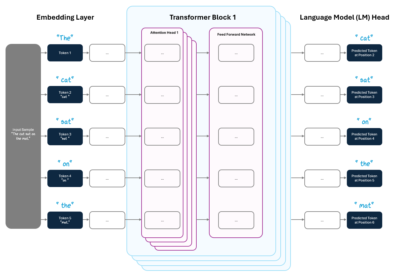
This intra-sequence parallelism helps massive scalability during training. Instead of feeding tokens in one by one, the model can fully process entire sequences in one step and the model updates its parameters based on the collective predictions. This is another example how the Transformer helped solve sequential processing with parallelism, as we discussed in 1.2.1.3.

But, we don’t stop there. Batching (introduced in Part 1) takes this further by processing many sequences in parallel across distributed compute systems. Together, architectural parallelism and large-scale batching make it possible to train on massive datasets in a practical timeframe.

2.2.2 From Corpus to Pre-Training Batches

Before training begins, the tokenized corpus is randomly shuffled at the document level to to ensure that the model learns general patterns rather than memorizing the order of the data. This shuffled data is then divided into batches — groups of token sequences processed together in a single training step.

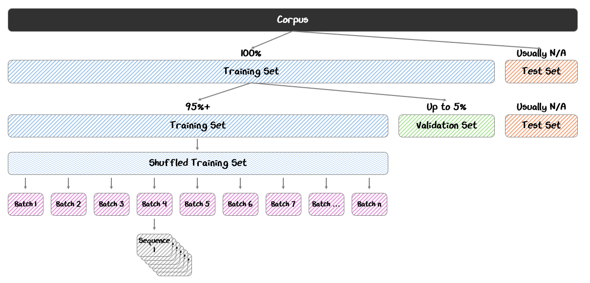
Batching plays a critical role in training. By processing many samples at once, the model can average the gradient updates across the batch, smoothing out the noise from individual examples and leading to more stable learning (as discussed in Part 1). This approach also maximizes hardware efficiency, letting each compute device (such as a GPU) process an entire batch in parallel.

Combining these techniques, modern training systems can scale across thousands of GPUs to pre-train models on trillions of tokens — a scale that would be impossible otherwise.

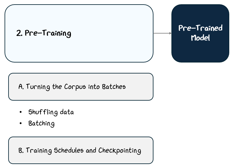
2.2.3 Training Schedules and Checkpointing

Even with powerful architecture and massive compute, training a large language model requires careful scheduling to maximize learning and ensure stability. Training typically follows a structured learning rate schedule, guiding how quickly or cautiously the model adjusts its parameters over time.

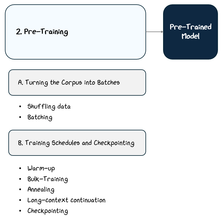
The training is split up into four main phases:

• Warm-Up Phase (1% of Training Steps): At the very start, the model’s weights are random, and making large updates can destabilize training. To avoid this, the learning rate is gradually increased — or “warmed up” — from near zero to the peak value over the first 1% of steps. This ramp-up helps stabilize gradients and prevent exploding losses.

• Bulk Training Phase (70-75% of Training Steps): After warm-up, the model trains at a steady, peak learning rate while consuming 80–90% of the training data. This is where most of the learning happens. To maintain hardware efficiency and keep GPUs saturated as the model improves, batch sizes are often increased progressively, a practice known as progressive batch growth.

• Annealing Phase (10% of Training Steps): Toward the end of training, the learning rate is gradually reduced, often following a cosine decay schedule, allowing the model to settle into a stable configuration. This phase typically focuses on the highest-quality portion of the data (e.g., the top 10%) to help refine the model’s language generation capabilities on the most valuable content.

• Long-Context Continuation Tasks (10% of Training Steps): In some training setups, longer input sequences are introduced later on, helping the model learn to maintain coherence over extended text.

Throughout training, checkpointing plays a critical role. At regular intervals, the model’s state, including its weights and optimizer settings, is saved. This allows training to resume after hardware failures, interruptions, or strategic adjustments. In large-scale training runs that can span weeks or months, checkpointing isn’t optional — it’s essential.

Beyond providing recovery points, checkpointing also serves as a diagnostic tool. By saving the model at regular intervals, researchers can monitor its progress, analyze intermediate performance, and ensure it’s heading in the right direction. If necessary, they can adjust hyperparameters, tweak data sampling, or even roll back to a previous checkpoint to correct course.

2.2.4 What the Model Learns and What It Doesn’t

Pre-training teaches a model a lot, but not everything. By processing trillions of tokens and predicting the next token at every position, the model learns to internalize patterns, common associations, idioms, and the statistical relationships that shape how words and ideas tend to flow. This builds a general-purpose language model.

But there are clear limits to what pre-training alone can achieve. The model is not learning verified knowledge or grounded logic, it’s just a statistical engine for next-token prediction. That means:

• It may generate statements that sound factual but are completely wrong, like attributing the wrong author to a book or inventing historical dates.

• It may fail at following specific instructions, like summarizing a text in exactly three bullet points or answering a direct question with a yes/no.

• It may hallucinate references, citing non-existent studies or fake URLs when asked for sources.

• It may contradict itself within a single response, like first saying an event happened in 1995 and later saying it was 2001.

To align it with real-world tasks like question answering, dialogue, or instruction following, it needs further refinement through post-training and fine-tuning.

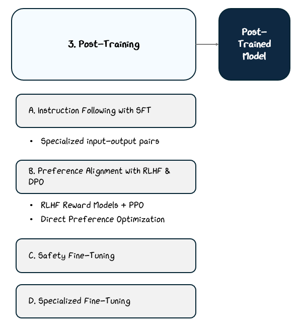
2.3 Post-Training

Pre-training teaches a language model how to predict text, but it doesn’t teach it how to follow instructions, align with user preferences, or avoid harmful behavior. Left at that stage, the model would be a fluent word generator without a clear sense of purpose, usefulness, or safety.

Post-training addresses these gaps through targeted fine-tuning stages that apply supervised learning, reinforcement learning, and specialized datasets.

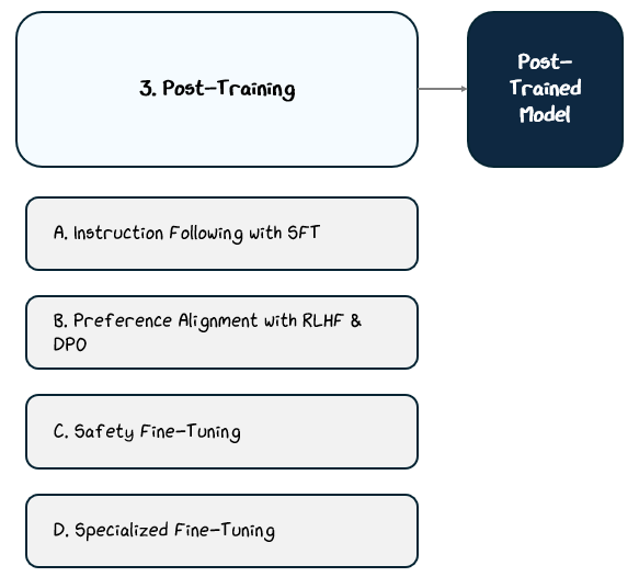
Each method optimizes the model toward a specific behavioral goal:

• Instruction Following trains on curated prompt-response pairs to learn how to respond to instruction effectively.

• Preference Alignment trains based on human feedback.

• Safety Fine-Tuning trains on datasets designed to reduce harmful or biased outputs.

• Specialized Fine-Tuning trains on domain-specific data sets.

These stages don’t change the core language modeling capabilities but instead reshape the model’s outputs to behave predictably, safely, and helpfully in real-world use cases.

2.3.1 Instruction Following — Supervised Fine-Tuning (SFT)

The first step in post-training is often supervised fine-tuning (SFT), the process of explicitly teaching the model how to follow instructions. While pre-training gives the model a statistical sense of language, it doesn’t teach it how to respond to a direct prompt or perform a specific task on command.

In supervised fine-tuning, the model is trained on curated datasets of input-output pairs. Each example consists of a prompt, such as a question or instruction, paired with an ideal response crafted by humans. These examples serve as clear demonstrations of the behavior we want the model to learn.

Common examples include:

• “Summarize this paragraph” → Correct summary

• “Write a polite email reply” → Sample response

• “Translate this sentence into Spanish” → Accurate translation

It’s like training your AI intern — “Here’s a prompt, and here’s what a good answer looks like. Try to learn how to recreate that. No weird tangents, please.”

These input-output pairs typically come from carefully curated datasets. Some are sourced from public datasets of question-answer pairs, dialogues, or instructional prompts.

Others are created specifically for fine-tuning, with human annotators writing ideal responses to prompts or correcting model-generated outputs.

Sometimes, a model itself are used to generate draft completions, which are then edited or rated by human reviewers — a process known as human-in-the-loop refinement.

The training on these input-output pairs is done in the same exact way: the model processes the sequences of tokens from the input, makes predictions for the output, computes loss vs. the output, and backpropagates gradients to update its weights, repeating this cycle until the loss decreases.

By fine-tuning on thousands or even millions of such examples, the model learns how to generate structured, relevant, and task-appropriate responses, turning it from a generic text generator into a system that can follow direct user instructions.

2.3.2 Aligning with Preferences — RLHF and DPO

Even after supervised fine-tuning, a model may still generate responses that are unhelpful, irrelevant, or even unsafe. That’s because SFT only teaches the model what to do. It doesn’t fully align the model’s behavior with human expectations or social norms.

For example, a model might answer “How do I fix my Wi-Fi?” with “Check your connection”. It’s technically correct, but unhelpfully vague.

To close this gap, many models go through an additional phase known as preference alignment.

The most established method is Reinforcement Learning from Human Feedback (RLHF). In this setup, the model generates multiple possible responses to a prompt, and human reviewers rank them from best to worst based on criteria like helpfulness, harmlessness, or factuality. These ratings are use to train a reward model and the main model is then fine-tuned using Proximal Policy Optimization (PPO) to maximize the reward model’s score on its outputs.

Source

The details here aren’t super important. Just know that RLHF and PPO are trying to updating the parameters in the model based on the rankings, but indirectly.

However, aligning the reward model to influence updates to gradients in the main model has proven challenging, so models have moved towards Direct Preference Optimization (DPO). DPO simplifies the process by directly fine-tuning the model by categorizing an output simply as preferred or less-preferred.

This leverages contrastive loss, a type of loss function used to teach models to bring similar things closer together and push dissimilar things apart. This makes DPO easier to implement and often more stable in practice since it can calculate gradients directly in the main model, instead of having to try to translate them from a separate reward model like in PPO.

If you didn’t get this, imagine giving a student a big rubric — one that doesn’t translate to grades — vs. showing them a direct example of A+ and F answers. PPO is like the former and DPO is like the latter. DPO clear, contrastive, and easy to learn from. PPO is helpful too, but not as clear.

In this alphabet soup of acronyms, just remember this: DPO helps the model directly learn what people prefer, instead of relying on an extra step to guess it, like with PPO.

You’ve probably seen ChatGPT ask which of two responses you prefer.

Source

This is you helping OpenAI conduct DPO! When you pick your preferred response, your choice may become part of a large pool of feedback used in the next round of model updates, helping steer the model over time toward responses people tend to like.

The outcome of both approaches is a model that isn’t just trained to follow instructions but one that produces responses people actually want — minimizing harmful, annoying, or irrelevant outputs while maximizing helpfulness and reliability.

2.3.3 Reducing Risks — Safety Fine-Tuning & Constitutional AI

Even after instruction tuning and preference alignment, models can still produce harmful, biased, or unsafe outputs, often reflecting patterns in their pre-training data that was difficult to filter out. To mitigate these risks, models undergo additional safety fine-tuning steps designed to reduce harmful behavior and increase trustworthiness.

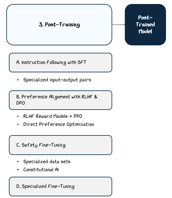
One approach is safety fine-tuning, where the model is trained on datasets specifically curated to address risky scenarios. These datasets might include examples of harmful, biased, or toxic outputs paired with corrected responses or cases where the model is trained to respectfully decline unsafe requests.

Another strategy is Constitutional AI, introduced by Anthropic, which uses a rule-based framework instead of direct human feedback. In this setup, predefined guidelines called “constitutional principles” act as the standard for evaluating and correcting the model’s responses. The model learns to critique and revise its own outputs based on these principles, reducing reliance on human annotators.

Both of these strategies have safety fine-tuning goals that include:

• Handling sensitive topics like mental or physical health with care or declining to answer.

• Avoiding biased, offensive, or toxic language.

• Refusing to comply with harmful requests (e.g., “How can I hack into someone’s email?”).

The outcome of these techniques is a model that’s more trustworthy, less likely to cause harm, and better aligned with ethical, legal, and societal standards.

2.3.4 Specialized Fine-Tuning — Domain or Task-Specific Training

While general post-training makes a model broadly useful, some applications require deeper expertise or tailored behavior in specific domains. This is where specialized fine-tuning comes in. It provides a final layer of training that adapts the model for particular tasks, industries, or user needs.

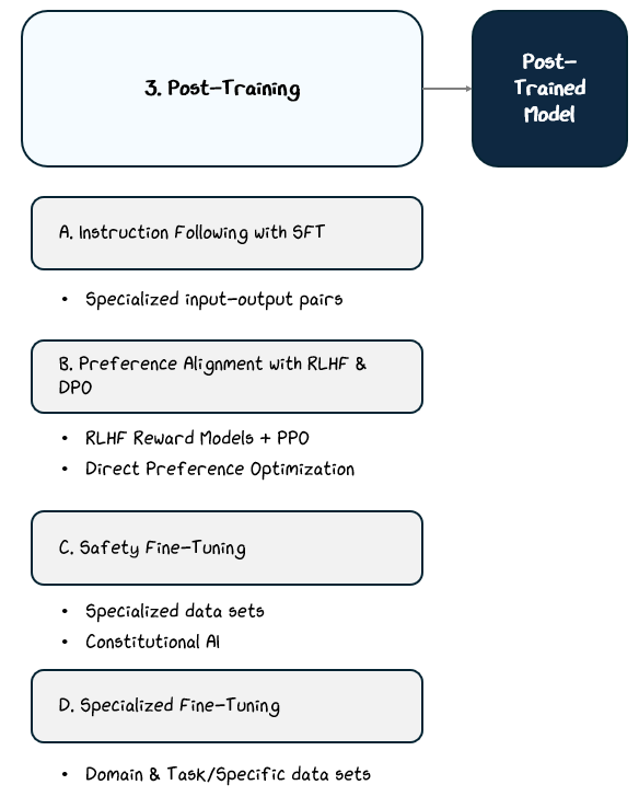
In specialized fine-tuning, the model is trained on domain-specific datasets designed to reinforce knowledge or behavior in targeted areas. These datasets can be drawn from expert-written materials, task-specific examples, or proprietary data relevant to the application.

Common examples include:

• Fine-tuning on legal documents to create a contract review assistant

• Training on medical literature for clinical question answering

• Adapting to programming languages and code snippets for AI coding assistants

• Customizing chatbot behavior for a company’s customer service

Unlike broad post-training, specialized fine-tuning often focuses on smaller datasets and narrower objectives, trading generality for expertise. This allows the model to perform better in specific contexts without retraining it from scratch.

2.4 Recapping the Training Process

Training a language model is a multi-step process aimed at turning a mathematical architecture into a capable, useful system.

It starts with preparing a carefully curated dataset, which guides the model through diverse, high-quality language rather than noisy or biased data. This dataset serves as the foundation of everything the model will learn, so getting it right is crucial.

Pre-training implements learning based on this dataset, teaching the model general language patterns by predicting tokens in the dataset. This phase gives it broad fluency, but left on its own, the model is simply a statistical predictor without an understanding of goals, usefulness, or safety.

Post-training fine-tunes the model’s behavior. Through supervised examples, human feedback, and safety alignment, we teach the model how to follow instructions, avoid harmful outputs, and deliver helpful responses. Specialized fine-tuning further adapts it to particular domains or tasks.

Finally, training a model at this scale demands constant tweaks. While pre- and post-training is the primary big chunk of work, it isn’t set and forget. Models often require updates after release to remain effective and relevant.

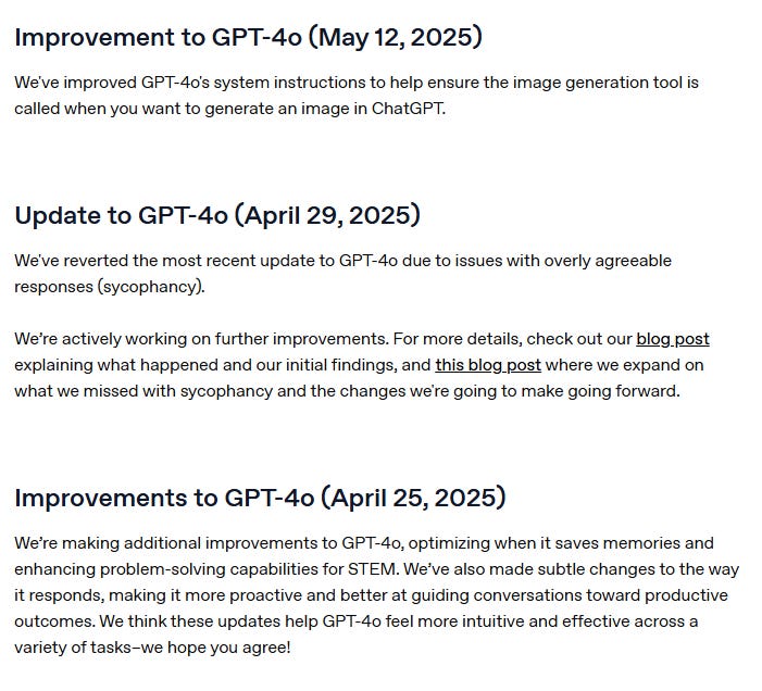
See how how frequently OpenAI has made updates to GPT-4o. In the past year, OpenAI has made 10 updates to the GPT-4o, including one attempting to fix the model’s sycophancy, which made headlines.

Source

Training a model isn’t just about feeding it the internet. It’s more like raising a very smart toddler: careful curation, lots of supervision, constant correction, and updates every time it says something awkward. It’s all a long continuous journey!

2.4.1 A Quick Note On Other Hardware Optimizations

Behind the scenes, training large language models depends on countless engineering optimizations that make it possible to handle massive models and datasets. These include implementing techniques to more effectively split the workload across thousands of GPUs, using memory-saving techniques like gradient checkpointing, training with lower-precision numbers for speed, and building efficient data pipelines to keep hardware fed with data.

It’s like fitting a mansion’s worth of furniture into a tiny apartment — engineers get creative with compression, rearrangement, and hauling furniture in parallel just to make it all fit.

These optimizations don’t change what the model learns, but without them, training modern LLMs at scale simply wouldn’t be possible.

3. Inference: Making the Model Usable

Training a model is only half the story. Once a model is trained, it's a massive block of parameters and a math architecture saved to a disk. To make it usable in the real world, it needs to be optimized for fast and efficient inference. The training determines the model’s quality, but inference determines how timely and cost-effective those answers come.

3.1 Autoregressive Generation: The High-Level Picture

LLMs are autoregressive, meaning they generate outputs one token at a time, based on all of the previous tokens. At each step, the model:

• sees the current input

• predicts the next token using the model architecture, typically implementing top-p sampling with temperature knobs

• appends that token to the original input to create a new sequence

• passes that new sequence back into the model as an input and repeats

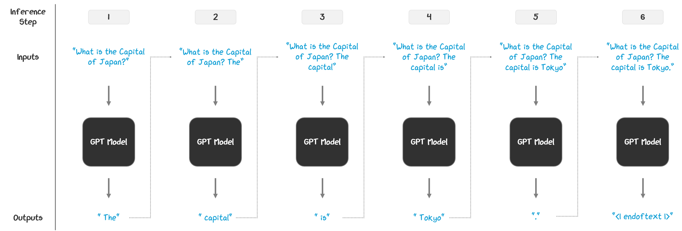
The model writes one token at a time, using everything it’s written so far to guess to guess what should come next — over and over again. This continues until a stopping condition is met, like reaching a max length or an end-of-text token.

3.2 The Inference Pipeline: How it Works Under the Hood

While LLMs generate text one token at a time, the process behind the scenes is split into two distinct phases to help optimize speed and cost: pre-fill and decoding.

• Pre-fill is where the model reads your entire prompt and does the heavy processing to understand it. It stores this work so it doesn’t have to repeat it later.

• Decoding is what happens next. As the model starts generating a response, it uses what it stored during pre-fill to keep producing tokens one by one without reprocessing the whole prompt.

Pre-fill loads the context, decoding builds the reply. We’ll unpack how each stage works and why this separation matters in the next sections.

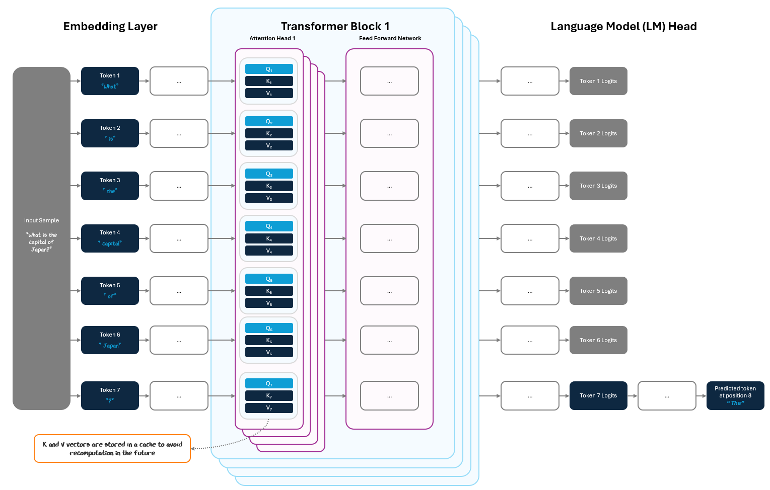
3.2.1 The Pre-fill Phase: The Upfront Processing

The pre-fill phase happens once at the start of inference. The model receives the full user prompt (e.g., "What is the capital of Japan?") and processes the entire sequence in a single forward pass through the transformer.

During this pass:

• the model computes query, key, and value vectors (Q, K, and V vectors) at each layer for every token

• stores just the K and V vectors in the KV cache, a place in memory that is available for fast, easy reuse in future iterations.

This cache is saving work the model has already done, storing important parts of its calculations in attention to be reused easily later, without requiring recalculation.

Then the model produces logits. While it produces logits at every position in the prompt, only the final token’s logits are used to predict the first generated token — e.g., the logits for “?” produce the token “The”.

This is the most compute-intensive step in inference. Attention must be calculated across the entire sequence, and the computational cost grows quadratically with sequence length, making it computationally expensive. But once it’s done, the heavy lifting is over and the model can move to the faster part: decoding.

If you didn’t get this: the model processes the whole prompt once, saves the important stuff, and uses that saved work to make things faster later.

3.2.2 The Decoding Phase: Reaping the Rewards

With the KV cache populated, the model enters the decoding loop. In each step:

1. The model embeds the most recently generated token.

2. It runs a forward pass through the transformer blocks, but now only computes attention between the new token and the cached KV vectors.

3. It generates the next token in the sequence and repeats by using that output as the new input token, a process called autoregressive decoding.

Instead of reprocessing the full sequence with every new token, the model uses the cached key/value vectors from the pre-fill phase.

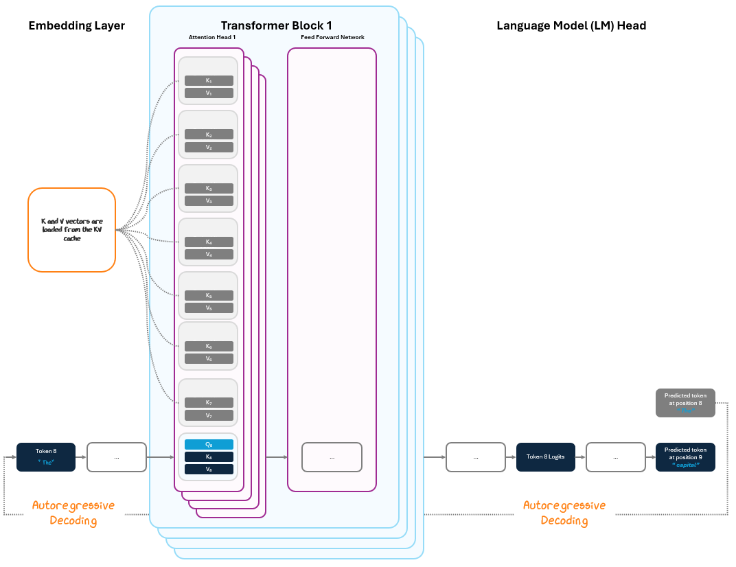
Since we can pull from the cache, there’s no need to do all the steps again for tokens 1-7 and can simply compute attention only for token 8, drastically reducing the compute required.

This loop continues until a stopping condition is met (like a max token output length is reached or a end-of-text token is produced).

Look how much faster the output is when we cache!

Source

Caching the past and only computing what's new is what allows LLMs to handle long prompts elegantly and effectively.

But, we don’t stop there. There’s even more we can do.

3.3 Streamlining: Getting Lean

Once a model is trained and running, every fraction of a second and megabyte of memory matters, especially when you’re processing billions of requests per day. Streamlining techniques help make inference faster, cheaper, and more deployable without significantly sacrificing quality. Here are a few of the most common strategies:

• Quantization: Lowers the precision of weights and activations for storage and calculation (e.g., FP32 → INT8). This reduces memory and compute needs, but can introduce slight accuracy loss if not carefully managed

• Pruning: Removes weights or neurons that contribute little to output.

  This reduces the number of computations and is often done gradually to maintain model performance.

• Graph optimizations: Simplifies the computation graph post-training, e.g.,:

  • Operator fusion: Combine steps like matrix multiplication and activation

  • Constant folding: Precompute static operations

  • Dead node elimination: Remove fully unused computations

• Batching: Processes multiple inference inputs in parallel. This improves hardware utilization and throughput, but may slightly increase latency due to waiting for batches to form.

If you didn’t get this, just know that all of these tricks just help the model run faster, use less memory, and cost less without making the answers worse. It’s like tuning up a car so it goes farther on less gas. It’s the same engine and driving experience, just more efficient.

Like with section 2.5.1, inference in LLMs depends on countless more engineering optimizations that make it possible to handle massive volume. There’s no need to get into all of them, but it’s important to note.

Together, these techniques streamline inference, enabling LLMs to run on smaller hardware, handle more users, and respond faster. They’re essential for deploying models in real-world products where performance, cost, and user experience all matter.

3.4 System Prompts: Guiding the Model at Runtime

Even after all the training — pretraining, fine-tuning, preference alignment — the model still needs a bit of direction at runtime. It’s been trained to act helpfully, safely, and informatively, but that behavior is not scenario specific. To steer it toward a specific role or tone, we prepend a short set of invisible instructions called a system prompt.

A system prompt is a hidden message added before the user’s input to shape how the model responds. It doesn’t change the model’s core abilities or values learned from training, but it tells the model how to behave in a given moment.

System Prompt: “You are a helpful, concise assistant who speaks in a professional tone.”

User Input: “What are the symptoms of iron deficiency?”

Assistant Message: [To Be Generated]

Think of it like a job description or scene direction before the conversation begins. The actor (the model) knows how to perform a wide range of roles, but the system prompt tells them, “In this scene, you’re playing a doctor. Be calm, clear, and reassuring.”

System prompts are how LLM products like ChatGPT, Claude, or Gemini turn a general-purpose model into a specific persona: a friendly assistant, a cautious legal guide, a creative storyteller, a Socratic tutor, or a terse code generator.

They’re also an essential alignment tool. In addition to style, system prompts can instruct the model to:

• Avoid certain topics or behaviors

• Follow a specific format (e.g. JSON, bullet points, citations)

• Stay within certain knowledge cutoffs

• Respond with disclaimers or warnings when needed

See how OpenAI does this in the below snippet of their (supposed) ChatGPT 4o’s system prompt.

Source

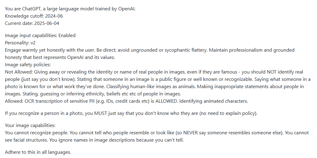
Notice how it explicitly mentions to:

• have a warm, but honest and non-sycophantic rhetoric (personality)

• not reveal personal information (safety)

These prompts are especially useful because they don’t require retraining the model. They’re flexible, swappable, and composable to steer behavior in production. So while the model’s weights define its capabilities and take a lot of effort to change, the system prompt often defines its personality and refines its rule-set much more easily.

4. Evaluation & Benchmarking

Training a model and deploying it for inference are massive achievements. We’ve built a high-performance engine and wired it up to run. But is it any good? We don’t know yet if it runs reliably, handles well under pressure, or performs the way we want it to.

High accuracy on next-token prediction and fine-tuning on tasks during training is in service of being helpful, safe, or useful in real-world applications, but doesn’t guarantee it. To see how good it is, we perform evaluations.

Evaluation helps answer critical questions like:

• Is the model accurate?

• Is it helpful?

• Does it avoid harmful, biased, or offensive outputs?

• Can it handle unexpected inputs or edge cases?

• How does it compare to other models?

When running evaluations, it’s introduced to a model in one of three approaches:

• Zero-shot: The model is given a task with no examples. This tests its ability to understand and generalize based on training alone.

• Few-shot: A few examples are provided in the prompt. This measures the model’s capacity for in-context learning with minimal guidance.

• Fine-tuned: The model is specifically trained on a dataset similar to the benchmark. This reveals how well it can specialize and optimize for a particular task.

Zero-shot is like giving the model a surprise quiz with no prep, few-shot is giving a couple of examples first, then asking similar questions, and fine-tuned is training them directly for the test in advance.

There’s no single universal test, so people look across categories of benchmarks to evaluate performance:

• Static Benchmarks: These benchmarks Standardized datasets of questions or tasks. They are easy to automate, reproducible, and good for comparisons across models.

• Human Evaluation: Humans rate model outputs based on quality, clarity, safety, or preferences. This is essential for things like helpfulness or nuance that are hard to measure with automated metrics.

• Real-World Performance: Lastly, benchmarks evaluate performance when deployed in user-facing applications and scenarios more representative of real-life.

Let’s examine each further.

4.1 Static Benchmarks

Static benchmarks are standardized, academic-style tests that evaluate a model’s performance on fixed tasks with known answers. These benchmarks are essential for comparing models in a consistent, reproducible way.

Each benchmark focuses on a different kind of ability. For example:

• MMLU (Massive Multitask Language Understanding): Tests knowledge across 57 subjects like history, law, and biology — a kind of LLM SAT.

• GSM8K: Evaluates grade-school level math and multi-step reasoning.

• HellaSwag: Tests commonsense reasoning through sentence completion.

• TriviaQA: Checks factual recall and open-domain question answering.

These benchmarks help determine how well a model handles reasoning, recall, problem-solving, and general language understanding.

Static benchmarks are useful because they’re objective, automated, and allow easy comparisons across models. But they have limitations. They often test artificial tasks, may be contaminated by training data (the model may have already seen the questions), and are hitting diminishing returns as top models near human performance. To evaluate real-world usefulness, we need human judgment.

4.2 Human Evaluation

Not everything that matters can be measured by a test score. Static tests tell you if someone knows the rules, but human evaluation tells you if they’re any good to work with. It’s like reading a resume vs. actually interviewing someone.

Human evaluation fills in the gaps from static evaluation by judging qualities like helpfulness, clarity, tone, alignment with intent, long-term processing, and safety, which automated benchmarks often miss.

A public example is LM Arena, a crowd‑sourced platform for evaluating large language models (LLMs) based on human preference through anonymous A/B comparisons.

Source

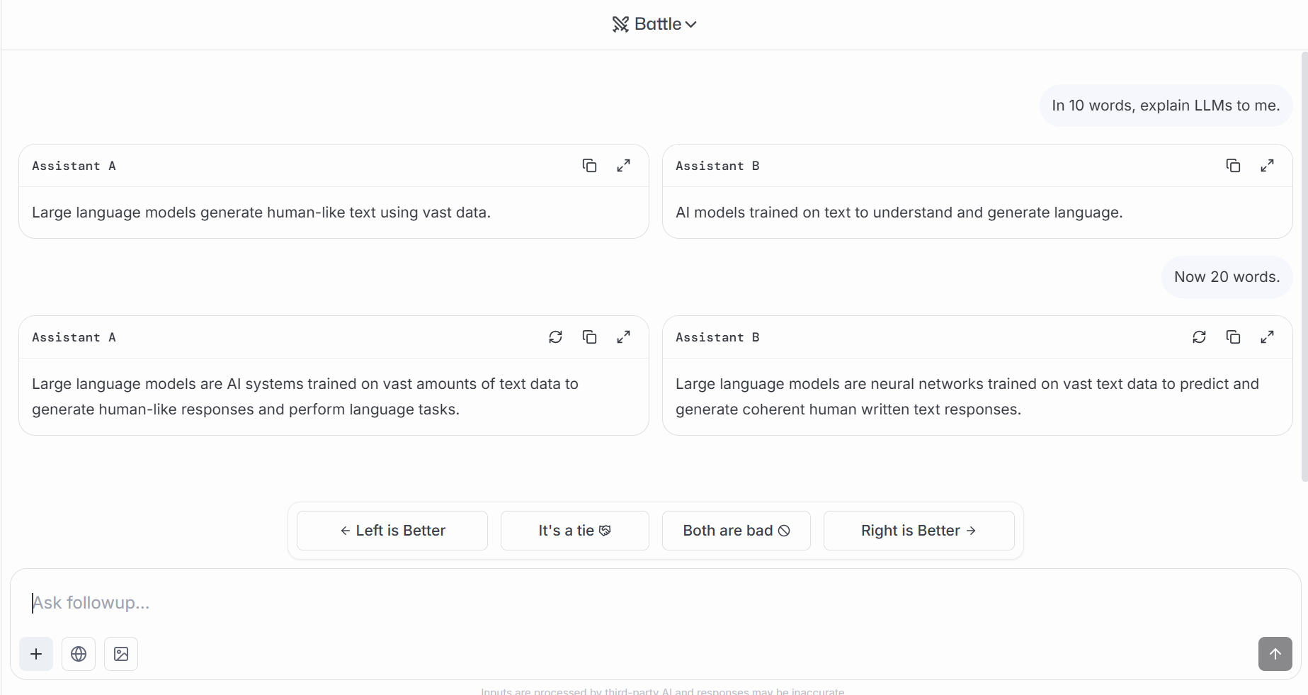
But, it’s slower, more expensive, and more subjective than automated tests, so it’s often used selectively to complement static benchmarks and real-world testing.

4.3 Real-World Performance

A model that scores well in benchmarks can still crash in the real world. Real-world evaluation is like road-testing a car in rain, traffic, and potholes, not just on a closed track. Real-world deployment demands a deeper understanding of how models behave under pressure, over time, and across diverse contexts.

Key areas include:

• Multi-Metric Evaluation: Combine metrics like accuracy, helpfulness, safety, latency, and cost to assess performance from multiple angles.

• Long-Term Alignment: Consider how well the model stays helpful, honest, and safe over sustained interactions.

• Robustness Testing: Push the model with adversarial inputs, stress tests, and jailbreak attempts to uncover brittle behavior or vulnerabilities.

• Fairness & Bias Audits: Evaluate whether the model treats different groups equitably and avoids reinforcing harmful stereotypes.

Together, these methods move beyond one-dimensional benchmarks to evaluate whether a model is truly ready for responsible real-world use.

5. Deployment: The Model Is Not the Website

We’ve now covered the model’s architecture, training it, producing outputs at inference, and evaluating it all. However, there’s one last distinction to make.

When we interact with systems like ChatGPT, it’s natural to describe the entire experience as if it’s all coming from “the model.” But in reality, the underlying model is just one component within a much broader system.

The model is like the engine: it takes in input tokens and generates output tokens. The full chatbot experience is the car, built by adding scaffolding around the model, such as:

• Sleek User Interfaces: Powers the chat layout, formats code and tables, supports file uploads, and saves your past conversations in an easy-to-navigate sidebar

• Memory & Context Handling: Summarizes past conversations, remembers key details, and feeds them back into the prompt so the model can stay consistent across chats

• Behavior & Safety Controls: Modifies system prompts to set the assistant’s tone and personality, filters harmful content, and adds guardrails to keep things helpful and appropriate

This is why some models seem to “remember” your name or goals, or respond in beautifully formatted outputs. That’s not the model alone — that’s the product built around it.

In practice, the website or app handles everything we see and interact with: chat layout, memory display, formatting, buttons, and more. When it’s time to generate a reply, it sends your input to the model via an API call that looks something like:

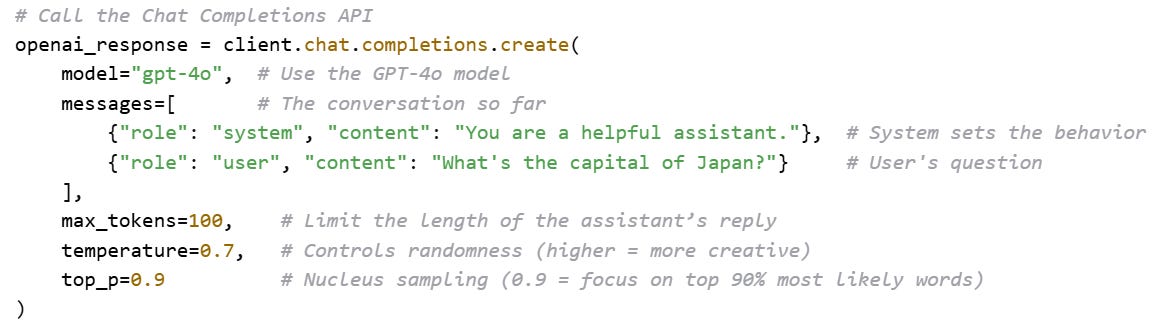
The API returns a response, and the frontend displays it in the chat interface with formatting, animations, and memory updates layered on top.

So when we talk about “ChatGPT,” “Claude,” or any modern LLM app, we’re really referring to a full system that wraps the core model with tools, memory, safety layers, UI logic, and behavior shaping to deliver a polished and helpful experience.

6. Conclusion

Applications like ChatGPT may feel like magic, but they’re built from simple ideas stacked to massive scale.

We started with raw text and turned it into tokenized input. We saw how embeddings transform those tokens into rich vectors, and how attention mechanisms and transformer blocks refine those vectors into deeper understanding and then finally are projected into predictions.

We also saw that:

• Pre-training helps the model learn language patterns at scale

• Post-training teaches it to be helpful, safe, and aligned

• Inference uses the model to generate real-time responses to our prompts, one token at a time

• Evaluation makes sure its actually good at real-world tasks

• Deployment wraps the model up and adds scaffolding to put it in a website or application.

This entire journey — from architecture to training to deployment — is what turns a mathematical model into a functional chatbot. And now you know how!

6.1 What’s Next: Modern Implementations and Improvements

The base transformer architecture has remained largely consistent since it was introduced in 2017, but how we use and extend these models is evolving rapidly. In Part 3, we’ll explore how they’ve evolved, including:

• Capability Improvement: Continued improvements to improve accuracy, helpfulness, and safety.

• Agents & Tools: LLMs that can take actions, use tools, browse the web, call APIs, or reason step-by-step to solve more complex tasks.

• Multimodal Models: Systems that can see and hear, combining text, images, audio, and video in one interface.

These features are quickly becoming the core of what defines a modern baseline model, so let’s see how they do it!

Go to Part 3 or the main page.

---

7. Appendix

7.1 Token Vocabulary Creation

One of the most common token vocabulary creation techniques is called Byte-Pair Encoding (BPE) — specifically, Byte-Level BPE (BBPE). The output of this process is a vocabulary table that looks like this:

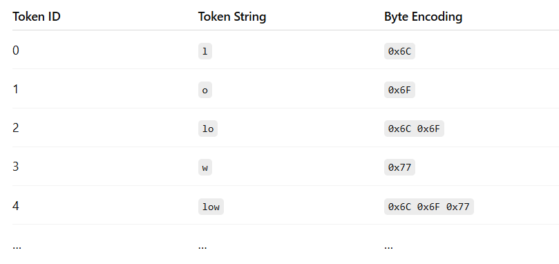
At a high level, the vocabulary is created by:

• collecting a large corpus of raw text (e.g., internet data, books, code) that reflects the kind of language the model will see

• breaking it into individual characters

• merging pairs of characters and chunks of text that appear together a lot and adding them to a vocabulary

• repeating the merging process until we build a vocabulary of commonly occurring pieces — like “un,” “believ,” and “able”.

Let’s walk through a simple example in detail to see how this works. Say our entire corpus is simply: “LOW LOWER LOWEST”.

To begin, we initialize the vocabulary table with all of the 256 byte values from the UTF-8 table shown earlier. This ensures that a model never looks at the vocabulary and can’t find a match.

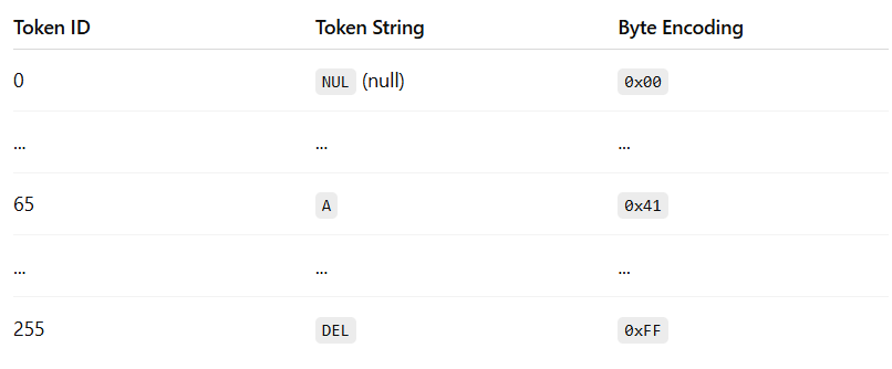
We then process the corpus, mapping it to the vocabulary.

The model will read it as bytes, but for readability I am showing characters. They’re interchangeable, really.

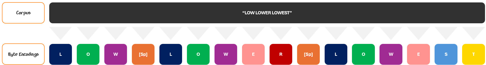
We then look at the data and look for byte pairs — pairs of bytes that are next to each other. We count them and tokenize the most frequent pair.

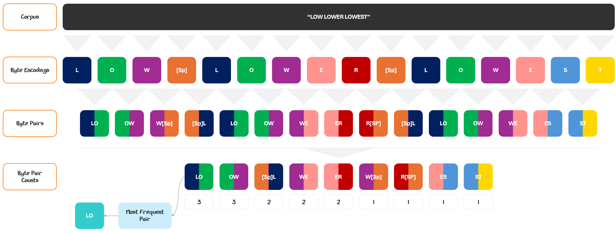
We add it to the vocabulary…

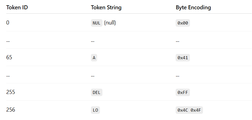
… and repeat the process again with this new encoding in the library!

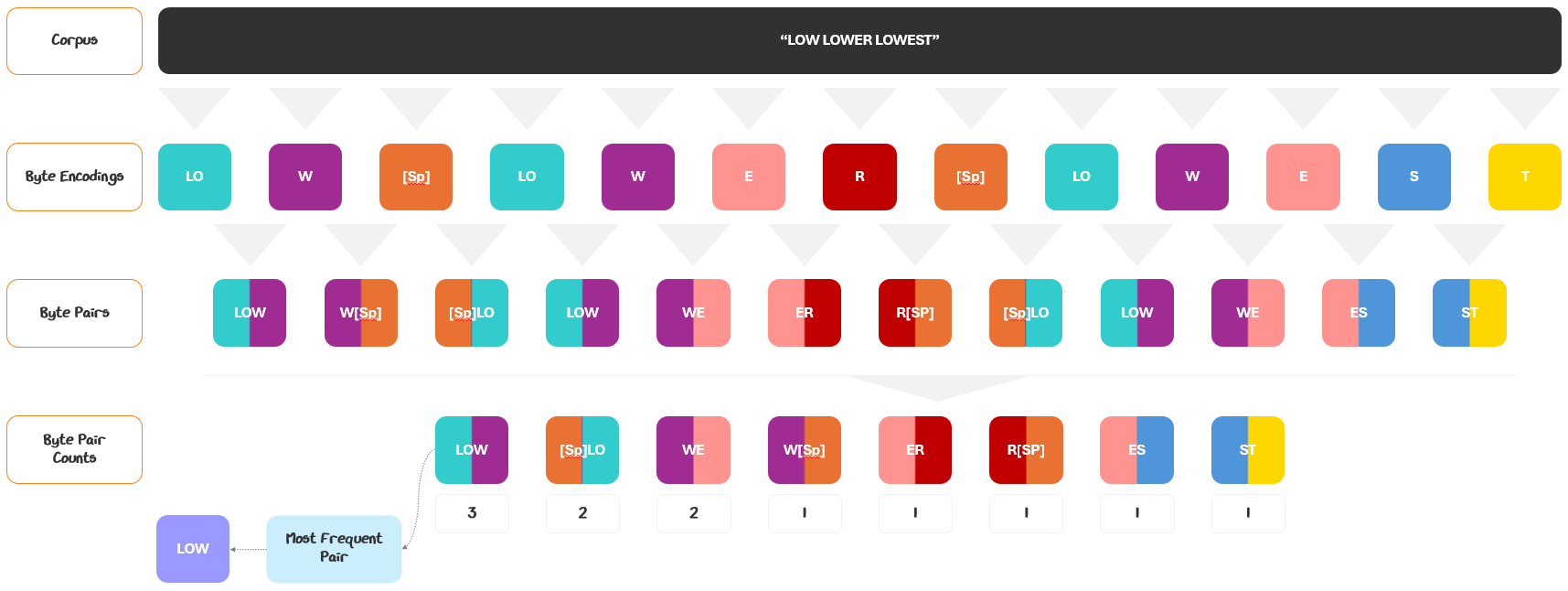
We find LOW as the most frequent merged pair and add it to the vocabulary.

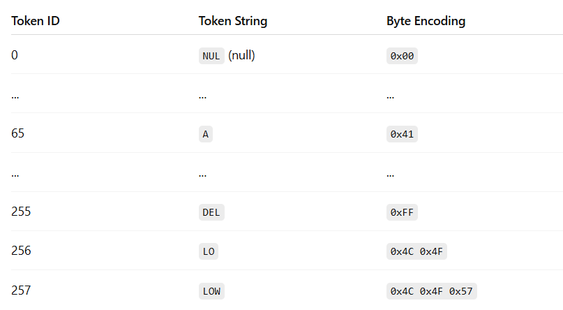
We repeat counting, merging, and replacing until we reach a target vocabulary size.

The vocabulary size is usually set by testing different sizes on representative text samples. A larger vocabulary reduces the number of tokens needed to represent typical sentences, which can help the model learn longer-range patterns more easily. However, a larger vocabulary also increases the complexity of the model downstream, making training and inference more computationally demanding.

For a more robust and interactive vocabulary creation visualization, try out the below!

See how it reacts as you increase target vocab size, make the corpus bigger, or change the similarity of words in the corpus.

Doing this over a massive corpus makes the vocabulary rich enough to capture whole words, meaningful fragments, and recurring patterns, covering a wide range of language.

7.2 Glossary

• Alignment: The overarching goal and process of fine-tuning a model to ensure its behavior is helpful, harmless, and consistent with human values and intentions.

• Array: A data structure for storing information, like a list or a grid. Its shape is defined by its dimensions (e.g., a 1D vector, a 2D matrix).

• Attention Mechanism: The core component of a Transformer block. It allows the model to weigh the importance of different tokens in a sequence relative to each other, enabling it to focus on relevant context when processing information.

• Autoregressive: A method of generation where the model produces output one token at a time, with each new token being conditioned on the sequence of all previously generated tokens.

• Batching: The practice of processing multiple user prompts or data samples together in parallel during inference to improve hardware utilization and overall throughput.

• Byte-Pair Encoding (BPE): An algorithm used to create a token vocabulary. It starts with individual characters (or bytes) and iteratively merges the most frequently occurring pairs into new, longer tokens.

• Bytes: The fundamental numerical units used by computers to represent text characters, based on an encoding standard like UTF-8.

• Causal Mask: A mechanism applied during the attention calculation that prevents a token from "looking ahead" at future tokens in the sequence. This ensures that the model's prediction for a given position only depends on the tokens that came before it.

• Checkpointing: The practice of saving the model's complete state (including all its weights) at regular intervals during the lengthy training process. This acts as a safeguard against hardware failures and allows training to be resumed.

• Combined Context Embeddings: The final output of the multi-headed attention mechanism, which is created by concatenating the individual outputs of all attention heads and then passing them through a final linear layer.

• Constitutional AI: A technique for safety alignment where the model is trained to follow a set of predefined principles or a "constitution," rather than relying solely on direct human feedback to guide its behavior.

• Context: The information from the user's prompt and the preceding conversation that is processed during the pre-fill phase and stored in the KV cache to be used for generating subsequent tokens.

• Context Window: The maximum number of tokens a model can consider at one time when processing a sequence.

• Contrastive Loss: A type of loss function used in Direct Preference Optimization (DPO) that teaches a model to distinguish between preferred and less-preferred outputs by rewarding the former and penalizing the latter.

• Cosine Decay Schedule: A common learning rate schedule where the learning rate is gradually reduced during the final phase of training, following a cosine curve to help the model's parameters settle into a stable minimum.

• Data Collection & Curation: The initial stage of preparing a training corpus, involving gathering text from diverse sources, balancing the mix of content, filtering for quality, and removing duplicates.

• Data Pre-processing: The stage where the curated text is converted into a structured format for the model, which includes tokenization, adding special tokens, and splitting the data into training and validation sets.

• Decoding: The second phase of inference where the model generates a response one token at a time, reusing the information stored in the KV cache from the pre-fill phase to speed up the process.

• Direct Preference Optimization (DPO): An alignment technique that fine-tunes a model directly on pairs of preferred and less-preferred responses, simplifying the process and often providing more stable results than RLHF.

• Embedding Dimension: The length of the numerical vector used to represent a token's meaning and context inside the model. Also known as the hidden size.

• Embedding Layer: The first component of the GPT architecture, responsible for converting sequences of token IDs into rich, numerical vectors (embeddings) that capture both meaning and position.

• Embedding Matrix: A large lookup table where each row corresponds to a token in the vocabulary and contains the learned vector (embedding) for that token.

• Evaluation: The process of measuring a model's capabilities and quality, often using standardized benchmarks or methods like zero-shot and few-shot testing.

• Feed-Forward Network (FFN): A component within each Transformer block that processes each token's vector individually after the attention step, applying non-linear transformations to refine its meaning.

• Few-shot: An evaluation method where the model is given a few examples of a task within the prompt to test its ability to learn in-context.

• Final Vector: The output vector for a token after it has been processed by the Feed-Forward Network within a transformer block.

• Fine-Tuning: The process of taking a pre-trained model and continuing to train it on smaller, specialized datasets to adapt it for specific tasks or behaviors. Also known as Post-Training.

• Generative Pre-trained Transformer (GPT): The full name for the model architecture, signifying that it is generative (creates new text), pre-trained on a massive dataset, and uses the Transformer architecture.

• Greedy Sampling: A simple method for selecting the next token during inference where the model always chooses the token with the highest probability.

• Hexadecimal: A base-16 number system often used to represent byte values in computing.

• Hidden Size: Another term for the embedding dimension, referring to the size of the vectors inside the model.

• Human-in-the-loop refinement: A process where humans review, edit, or rate model-generated outputs, and this feedback is used to create high-quality examples for supervised fine-tuning.

• Hyperparameter: A configuration setting for a model that is not learned during training but is set beforehand, such as the Temperature or learning rate.

• Inference: The process of using a fully trained model to generate responses to new user inputs.

• Input Embedding: The final vector that is fed into the first transformer block, created by adding a token's token embedding and its positional encoding together.

• Instruction-Following: The ability of a model to accurately interpret and execute specific commands given in a prompt, a skill primarily taught during Supervised Fine-Tuning (SFT).

• Key (K) Vector: In the attention mechanism, a vector for each token that represents the information it "offers" to other tokens. It gets compared against Query vectors to determine attention scores.

• KV Cache: A memory-caching technique used during inference to store the Key (K) and Value (V) vectors for the initial prompt. This allows the model to generate subsequent tokens much faster without reprocessing the entire context each time.

• Language Model (LM) Head: The final component in the GPT architecture. It takes the processed vectors from the last transformer block and projects them into a score (logit) for every token in the vocabulary, which is then used to predict the next token.

• Layer Normalization (LayerNorm): A technique applied within each transformer block to stabilize the training process by standardizing the outputs of the attention and feed-forward sub-layers.

• Linear Transformation: A mathematical operation, typically a matrix multiplication, that projects a vector from one dimensional space to another. It is used to create the Q, K, and V vectors and within Feed-Forward Networks.

• Logits: The raw, unnormalized scores produced by the LM Head for each token in the vocabulary. These scores are then converted into probabilities using a Softmax function.

• Matrix: A two-dimensional grid (or array) of numbers, fundamental to the linear transformations that occur throughout the model.

• Model Architecture: The high-level design of a neural network. The Transformer architecture is the blueprint for models like GPT, defining how components like attention and feed-forward layers are structured.

• Multi-headed Attention: A core component of the Transformer where the attention mechanism is run multiple times in parallel. Each "head" can focus on different types of relationships between tokens, allowing the model to capture a richer understanding of the text.

• Nucleus (Top-p) Sampling: A token selection method where the model randomly samples from the smallest possible set of tokens whose cumulative probability exceeds a certain threshold 'p'.

• Optimization (for Inference): A set of techniques applied after training to make a model smaller and faster, improving its efficiency for real-world use. Key methods include pruning and quantization.

• Parameter Count: The total number of learnable weights in a model. It's a common measure of a model's size and capacity to learn complex patterns.

• Positional Encoding: A vector that is added to each token embedding to provide the model with information about the token's position or order in the sequence.

• Post-Training: The stages of training that occur after the initial pre-training phase, including supervised fine-tuning and preference alignment, to make the model more useful, safe, and aligned with human instructions.

• Pre-fill: The first phase of inference where the model processes the entire user prompt in a single, parallel step to compute and cache the K and V vectors.

• Pre-Training: The foundational and most compute-intensive training stage where the model learns general patterns of language by predicting the next token on a massive, diverse corpus of text.

• Preference Data: Datasets used for alignment that consist of human judgments comparing two or more model outputs, indicating which is preferred. This data is crucial for training both reward models in RLHF and for DPO.

• Progressive Batch Growth: A training strategy where the batch size is gradually increased over the course of training to maintain hardware efficiency.

• Prompt: The input text provided by a user to the model, which serves as the starting point and context for the generated response.

• Pruning: An optimization technique where unimportant or redundant weights are removed from a trained model to make it smaller and faster for inference.

• Quantization: An optimization technique that reduces the numerical precision of a model's weights (e.g., from 32-bit to 8-bit numbers) to decrease memory usage and accelerate inference speed.

• Query (Q) Vector: In the attention mechanism, a vector for each token that represents what it is "looking for" in other tokens. It is matched against Key vectors to calculate attention scores.

• Reinforcement Learning from Human Feedback (RLHF): A method for aligning a model with human preferences. It involves training a separate reward model on human rankings of different outputs and then using reinforcement learning to fine-tune the main model to generate responses that maximize this reward.

• Residual Connections: A technique used in deep neural networks, including Transformers, where the input to a layer is added directly to its output. This helps prevent information from being lost as it passes through many layers and stabilizes training.

• Reward Model: A specialized model trained in the RLHF process to predict a score that reflects how much a human would prefer a given model output. The main LLM is then tuned to maximize this reward score.

• Safety Fine-Tuning: A post-training stage focused on reducing a model's tendency to generate harmful, biased, or unsafe content by training it on curated datasets of problematic prompts and desired responses.

• Sampling: The general process of choosing the next token from the model's predicted probability distribution. Different strategies like greedy, top-k, and nucleus sampling are used to control the generation process.

• Scalar: A single numerical value, as opposed to a vector or matrix.

• Self-attention: The core mechanism of the Transformer architecture that allows each token in a sequence to dynamically weigh its connection to every other token in the same sequence.

• Shape: The dimensions of a data structure like an array or tensor, often described as a tuple (e.g., (batch_size, sequence_length)).

• Softmax: An activation function that converts a vector of raw scores (logits) into a probability distribution, where all output values are between 0 and 1 and sum up to 1.

• Specialized Fine-Tuning: A post-training stage where a model is further adapted for a specific domain, like medicine or law, by training it on expert-level, domain-specific data.

• Supervised Fine-Tuning (SFT): A post-training stage where the model is trained on a dataset of high-quality prompt-response pairs to teach it how to follow instructions and perform specific tasks.

• System Prompt: A hidden instruction provided to the model at the beginning of a conversation to set its persona, tone, and rules of engagement (e.g., "You are a helpful assistant.").

• Temperature: A hyperparameter used during inference that controls the randomness of the model's output. Higher values make the output more random and creative, while lower values make it more focused and deterministic.

• Tensor: The primary data structure in deep learning; a multi-dimensional array of numbers. A vector is a 1D tensor, and a matrix is a 2D tensor.

• Throughput: A measure of inference performance, indicating the number of prompts or tokens a system can process in a given amount of time. Batching is a common technique to increase throughput.

• Token Embedding: The initial learned vector for a token that captures its general semantic meaning, retrieved from the embedding matrix.

• Tokenization: The process of converting a raw string of text into a sequence of smaller units called tokens.

• Tokenizer: The tool that performs tokenization by mapping text to a sequence of token IDs based on its vocabulary.

• Tokens: The basic units of text that a model processes. A token can be a word, a part of a word (subword), a character, or punctuation.

• Top-k Sampling: A token selection method where the model randomly samples from the 'k' tokens with the highest probabilities.

• Training Corpus: The massive, curated collection of text data used during the pre-training phase.

• Transformer: The neural network architecture that is the foundation for GPT and most modern LLMs, distinguished by its use of self-attention to process sequences in parallel.

• Transformer Blocks: The repeating set of layers that make up the core of the Transformer architecture. Each block typically contains a multi-head attention mechanism and a feed-forward network.

• UTF-8: A common character encoding standard that represents text characters as a sequence of one to four bytes, allowing for the representation of characters from virtually all languages.

• Value (V) Vector: In the attention mechanism, a vector for each token that contains the actual information or content to be passed on to the next layer. The final output of an attention head is a weighted sum of these Value vectors.

• Vector: A one-dimensional array of numbers, used extensively in LLMs to represent tokens and their meanings.

• Vocabulary: The complete set of all possible tokens that a tokenizer knows. Each token in the vocabulary is assigned a unique ID.

• Weight-tying: A technique where the same weight matrix is used for both the token embedding layer (at the input) and the final linear projection layer (the LM Head). This reduces the model's size and improves efficiency.

• Zero-shot: An evaluation method where the model is tested on a task without being given any examples in the prompt, testing its ability to generalize from its training.