A Semi-Technical Primer on LLMs: Pt. 1 How Machines Learn
Understanding fundamental Machine Learning concepts to use as building blocks in future parts.


To learn how ChatGPT can produce Shakespearean-esque literature on a whim, we must first understand how machines can solve much simpler tasks.
Feel free to skip this section and go straight to Part 2 if you already know how neural networks work but, even still, a quick refresher may not hurt.
Naturally, there is a bit of jargon in here. To help navigate this, words in bold are defined / clarified in a glossary at the end of each part.
1. Supervised Learning: Teaching by Example
At its core, most machine learning is about mapping inputs to outputs using examples. You give the model some input features (e.g., square footage and number of bedrooms in a house) and the correct output (e.g., the house’s price). The model sees these labelled samples and learns a mapping that minimizes a loss (how far off it is from the right answer). Feed it enough examples, and the model implicitly “learns” a rule for mapping A → B.
1.1 Fitting a line
Let’s start with the simplest form of supervised learning: fitting a straight line through some noisy data points — a linear regression.

A linear regression is powerful because you can make predictions by plugging in inputs to the mapping.
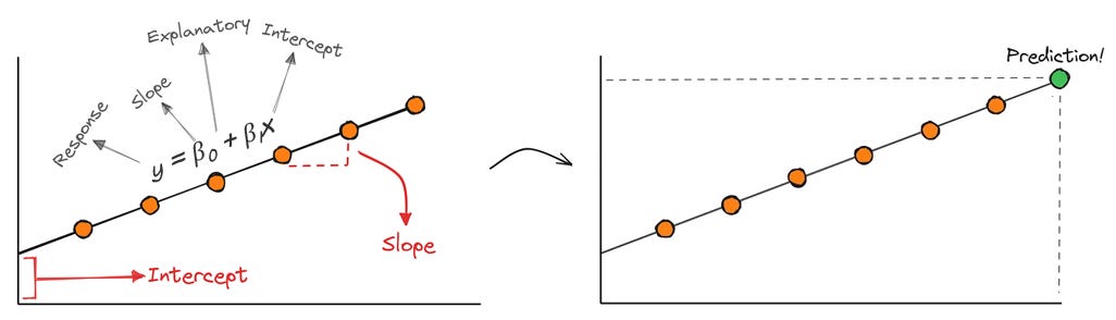
Suppose you're trying to predict housing prices using just one feature: square footage. In this case, the model is trying to find the right slope and intercept so that:
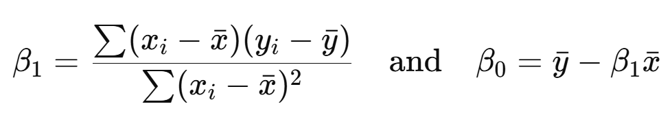
You likely learned how to mathematically solve this in school using formulas to find the coefficients through algebra:
Instead, machines learn the mapping through smart trial and error, since it scales better as the mappings become more complex.
To find the best slope and intercept by trial and error:
Your model makes predictions
You measure how wrong they are
You change the slope and intercept to lower the error
Repeat until you are happy with the predictions / loss!

1.1.1 Coming Up With Predictions
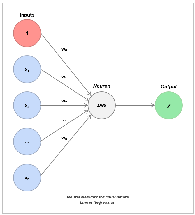
To do this in practice, we recreate the regression in a neural network:
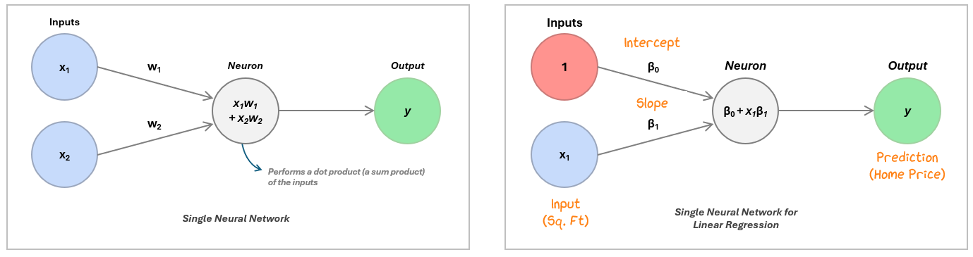
The neuron ingests the inputs, multiplies each one by a corresponding weight, and then adds them all together — this is called a dot product.
In linear regression, we include a special input of 1 (called the bias term) whose weight is the intercept. The other input is the actual feature, like square footage, weighted by the slope. The neuron calculates this weighted sum to produce its output — the predicted value, like a home price.
To come up with our prediction, we plug in the data points and see what the model outputs.
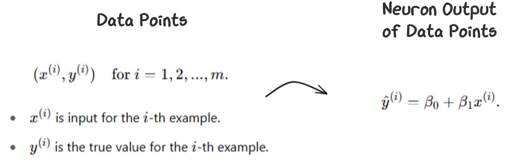
1.1.2 Measuring Error with Loss Functions
We then compare the predictions (ŷ) and actual values (y). To do this, we use a loss function, a formula used to calculate the error (the distance between the dots and the line):
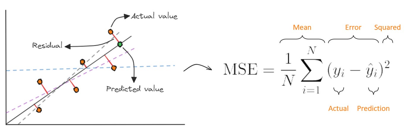
For linear regressions, we can use Mean Squared Error, which takes the error from each data point vs. the prediction, squares it, and averages across all data samples. This has some nice properties:
it's always positive (positive or negative misses don’t cancel each other out)
bigger mistakes hurt more (makes sure we’re never too far off)
the equation is differentiable and smooth (doing math to minimize error is easier)
1.1.3 Updating The Model via Gradient Descent
But, knowing how far our line is off is just step 1. We need a way for the model to find the better lines. That’s where gradient descent comes in: a systematic way for the model to adjust its parameters, little by little, to reduce the error.
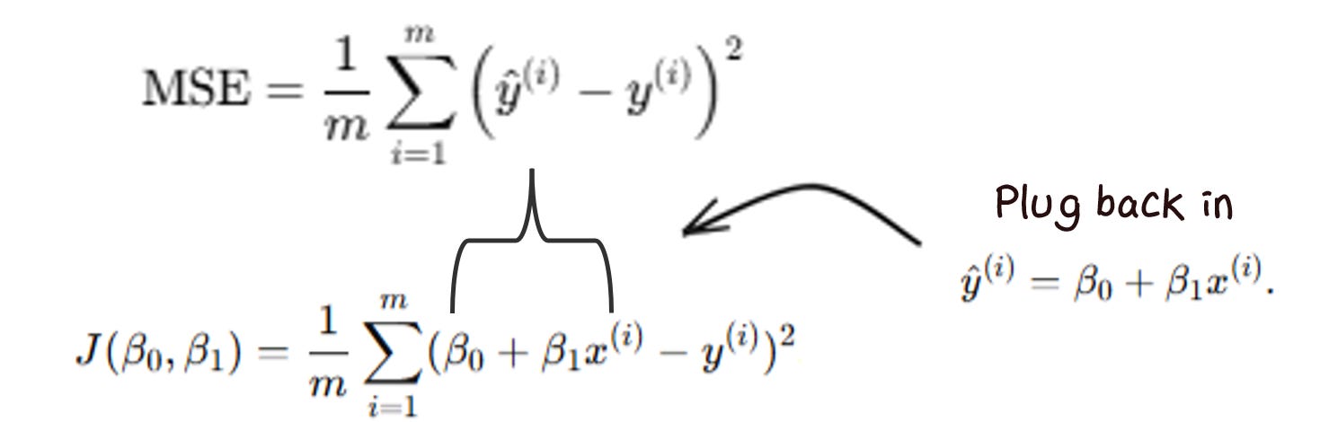
To do this, we get the equation in terms of the coefficients (slope and intercept) by plugging in ŷ.
We then take the partial derivatives of that new loss function, to get the gradient functions.
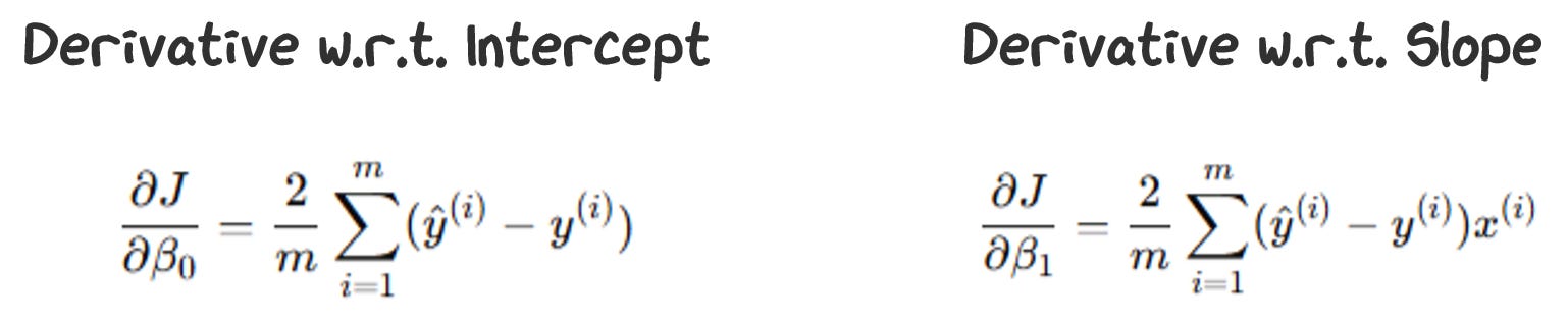
Plug in the predictions (ŷ) and actual values (y) to get the gradient. The gradient tells us:
which direction to move the weights to make the error smaller
how big a step to take
We update the weights based on this gradient, but adjust it by a learning rate. This makes sure we don’t adjust the weights too much or little — more on this soon.
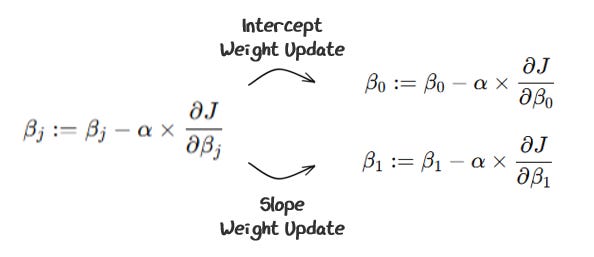
1.1.4 Completing A Training Step
This process can be summarized below.
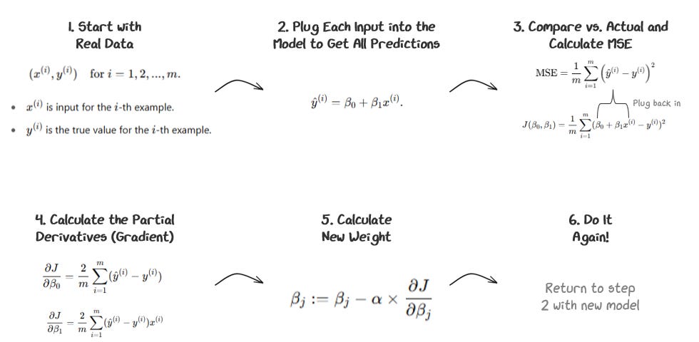
Each full cycle of steps 1-6 is a training step. You repeat this process, running training steps until you are happy with the predictions!
If you didn’t get the math portion, don’t worry. The idea is this: the model makes a guess, checks how wrong it was, and then adjusts itself to do a little better next time.
Think of the loss function as the landscape, the gradient as the slope of the terrain, and gradient descent as the model’s way of feeling its way downhill in the dark. You feel around for the downhill gradient and take a step downhill. You stop and reevaluate where you are, once again feel for the downhill gradient, and take a step, repeating this until you are at the bottom. When you are at the bottom, you’ll be pretty good at predicting!
1.1.5 Modifying Training Steps
The learning rate controls how big the steps we take are — i.e., how big each weight update is during each step of training. If it’s too big, the model might overshoot and diverge (you might jump and miss the hill entirely). If it’s too small, you might get stuck in bad local minima (you may never step far enough to find the hill).

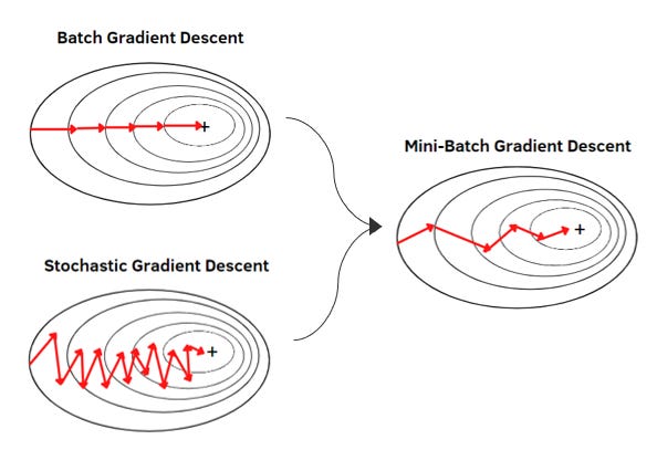
The example we mathematically walked through calculated the gradient descent for the entire data set in one go (since we summed up all of the errors across all data points). This is called a batched gradient descent. Since this requires performing the calculation for the entire data set, batch gradient descent can be very slow and impractical for larger data sets.
On the flip side, you can update the gradients after reading every new data point one at a time. This results in fast updates and randomness that helps escape local traps. However, this is super noisy and each step bounces around the true gradient direction. In our dark downhill example, this is like taking a step after glancing at just one tiny patch of ground. Sometimes the slope in that patch points you in a good direction. Sometimes it misleads you.
As a compromise, you can use mini-batches, taking 32, 64, 128, etc. data points at a time — not looking at just a tiny patch nor fully surveying the entire terrain, but looking in a good, representative general direction. This is the standard approach as it balances hardware limitations while reducing noise.
1.1.6 Putting it All Together In A Training Cycle
When you perform enough steps of mini-batches to have looked at all the data points, you have completed one epoch. For increased accuracy, you may train the model for multiple epochs. When you are fully done, you have finished your training cycle.
Putting everything together, we visually see how the line fits to the data points below:
The model initializes with random weights (-3.21 intercept, 3.16 Slope) — super wrong. We have it step through once (with a learning rate of 0.1 and batch size of 100 data points). It calculates a -4.47 gradient for the intercept (the green line) and a +38.08 gradient for the slope (the blue line) and scales them by the learning rate to get the new intercept and slope of -2.77 and -0.64, reducing the loss. Then we repeat!
On the right you can see how the weights are following the gradient “downhill”. The model takes big steps when its far away from the bottom since it’s steep and smaller steps as it hones in on the bottom.
Play around with the model! See how adjusting the learning rate, batch size, etc. adjusts the way the model “learns”.
1.2 Adding More Features for Multivariable Regression
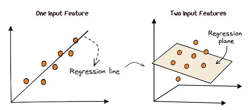
In the real world, we rarely have just one input feature. Let’s go back to our housing market example. A house price depends on square footage, number of bedrooms, zip code, and so much more.
To do this, we use multivariable linear regression. The idea is the same, but instead of fitting a line, you fit a higher-dimensional surface (e.g., a 2-d plane for two inputs).
In the neural network, you simply just add more inputs and weights into the neuron.
And predict using:
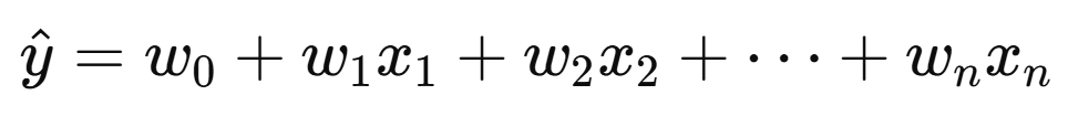
The goal is still to find the weights that minimize the loss, just now with multiple coefficients. We use gradient descent just like before to update each of the weights. Nothing really changes!
1.3 Preventing Overfitting With Regularization
When you have many weights, you can start to risk the model “overfitting”, learning noise, outliers, or quirks in the training data instead of the more generalized patterns.

To solve overfitting, you can make sure that weights don’t get too large by adding a regularization loss to the total loss.
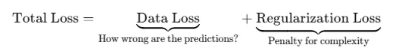
Two main types of regularization are used.
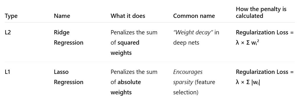
L2 (Ridge) penalizes large weights to reduce overfitting and L1 (Lasso) can zero out unnecessary weights, making the model simpler. Typically both are used in the model.
1.4 Adding Non-Linearity with Logistic Regression
Linear regression models a continuous outcome. But, sometimes we don’t want to predict how much. We want to classify something (e.g., is a credit card transaction fraud or not fraud?). A linear model can output any number, but we need the output to be more binary.
To achieve this effect, we wrap the linear prediction in an “activation function” called the sigmoid function.
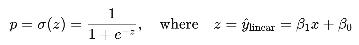
This function effectively squishes the linear regression output:
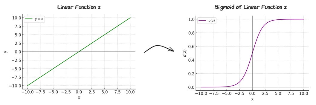
The sigmoid is a soft yes/no switch. It bends a straight line into a probability between 0 and 1. The output indicates how confident the model is that the label belongs to category 1. This means if p > 0.5, we are predicting category 1 and if p < 0.5, we are predicting category 0.
For logistic regressions (classification) MSE is not a great loss function. Instead we use cross-entropy loss (also called log loss).
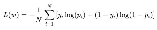
Cross-entropy loss measures how far off a model’s predicted probability is from the actual answer. It particularly rewards confident, correct predictions and heavily penalizes confident, wrong ones. This is useful for classification problems because it pushes the model to assign high probabilities to the right answers, not just get the answer right by chance.
Unlike linear regression, there’s no closed-form solution because the sigmoid makes it non-linear, so we must (!) use gradient descent to compute loss. When doing so, we follow the same high level steps: predict probability p, compute the loss, compute the gradients, and update the weights.
This is a little more complicated mathematically, since your loss doesn’t directly depend on the weights. Thus, you use the chain rule:
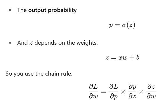
We’ll spare ourselves the rest of the math, but note that this chain rule allows more complicated neural networks to learn. We’ll come back to this.
Overall, we can see how this comes together, below:
Just like in linear regression, we’re initializing our model with default weights and stepping through gradient descent. But this time, instead of predicting a continuous number, we’re predicting the probability that a number is positive.
Finally, let’s add this activation function to our neural network!
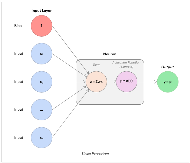
When you wrap a linear prediction in an activation function (e.g., a sigmoid) you get a single, decision-making unit: a perceptron. Just one is fairly simple, but stack them together, and you have the foundation of a neural network.
1.5 Identifying More Complex Patterns with a Multi-Layer Perceptron
One perceptron can only slice data with a straight line coming to simple decisions like yes or no, but real-world patterns, like determining credit card fraud, are more complicated.
One way of solving this is not just by adding more features / inputs, but by stacking neurons in horizontal layers. By stacking layers, you let the network build up more complex rules: e.g., the first layer might spot simple red flags like a high amount or an out-of-city transaction, the next layer could combine them — like high amount and out-of-city and swipe — and so on, until it’s capturing patterns you’d never spot on your own.
This stacking is called a Multi-Layer Perceptron (MLP), which contains an input layer with raw features, hidden layers, and an output layer with the final prediction.
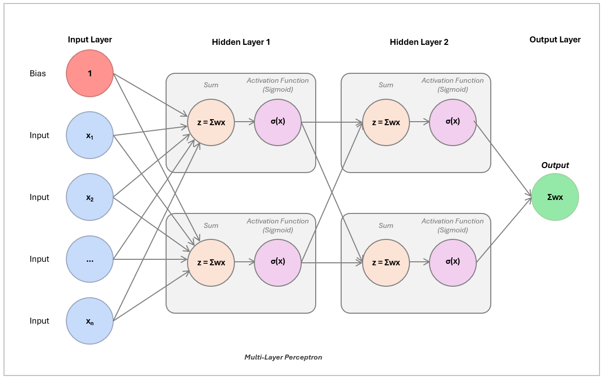
This is particularly powerful with the activation function, because the non-linearity adds much more ability to find non-linear patterns. Without it, you still just have a more sophisticated line generating machine.
To update the weights, we follow the same high-level steps: make a prediction, calculate the loss, compute the gradients, and update the weights. Remember the chain rule we discussed earlier? It’s what allows information to flow backward through the layers so we can adjust the weights at every step. This process of passing gradients backward is called backpropagation is what powers training with gradient descent for multi-layer models.
Here you can see the MLP’s ability to identify more complex patterns. Watch how it learns to classify the orange and blue dots, which are placed in highly non-linear patterns.

Each input feature (like x₁ and x₂) feeds into a layer of neurons, which combine and transform the inputs using learned weights. The outputs of this first layer pass through another layer, and finally to the output. The thickness of each line shows how strongly a neuron’s output influences the next layer (its weight). Some connections are weighted heavily, others barely contribute.
This is what powers neural networks. By stacking layers and adding non-linear activations, the collective power can learn to capture complex, abstract patterns in data.
1.6 A Note on Activation Functions
As mentioned, the activation function (the sigmoid function in our logistic regression) is key to making the model smart. Without it, no matter how many layers of neurons you stack, a neural network is just a fancy version of linear regression. Every layer would just be multiplying and adding numbers in a straight line. You’d never be able to capture complex patterns like curves, categories, or logic rules.
The activation function solves this by adding non-linearity — a way to bend or squish the output at each neuron, letting the network learn more intricate behaviors.
The activation function:
takes the weighted sum of inputs into a neuron
applies a mathematical function that changes that value in a predictable way
decides whether or not the neuron “activates” (influences the next layer)
We used a sigmoid function above, but this is just one of many activation functions! You don’t need to memorize every activation function, but here are some of the key ones, particularly because they are used to directly shape the output of a neural network.
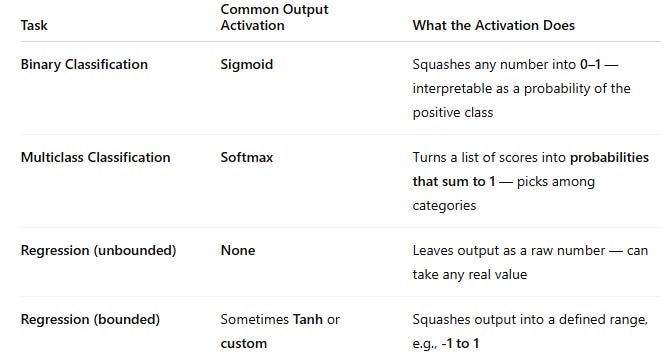
This article is great for learning more about the types of activation functions used.
2. Unsupervised & Self-Supervised Learning: Learning On Its Own
In classic supervised learning, you feed the model an input and a human-provided label. “Here is an input (square footage) and we are explicitly telling you the price is $1,000,000 (output)”. The output “label” provided by the human tells the model the correct answer, hence providing “supervision”.
This means you need to label a lot of data. This is slow and expensive!
2.1 Unsupervised Learning: Finding Patterns
Because of this, people started to explore unsupervised learning — finding patterns without explicit output labels. Instead of telling the model the specific “right answers,” you let it more abstractly find patterns.
For example, you don’t explicitly tell the model to discern between cats and dogs, but instead direct it to cluster the data into groups with similar patterns. Following this instruction, the model splits the data into two groups that look similar. The model is effectively sorting the data into cats and dogs, but without that explicit instruction, finding the differences on its own.
In the animation below, there is no one telling the algorithm that certain dots are yellow and certain dots are red. It’s more generally looking to categorize the random dots into two groups.
The process is just like supervised learning. You still have a predictive model and a bespoke loss function that you can perform a gradient descent on. For clustering similar groups together, the loss function is sum of distances from each point to its cluster’s center.
While the output is structured data (e.g., distinct clusters) and that can be useful, they are abstract since they don't explicitly define output labels and give the groups meaning. You still have to figure out that the model created a cluster of dogs and a cluster of cats by examining the clusters yourself.
2.2 Self-Supervised Learning: Making Those Patterns Useful
So people started to ask: can we trick the model into training itself to tell us the labels? This gives you all the benefits of supervised training — strong loss functions, gradient descent, clear outputs — without paying people to label millions of examples and without the vagueness of unlabeled outputs.
To do this, you implement a neat trick: create the label from the data itself by hiding part of the input and making it the output label. For the data point “The cat sat on the mat.” The model input is “The cat sat on the ___.” The output label is “mat.” If the model predicts “mat”, loss is low. If it predicts something else, loss is high.
The whole loop is just like classic supervised training except nobody typed ‘mat’ as target output label. The data contains the answer — take a sentence and hide a word and now “guess the missing word” becomes the training signal. This trick turns the entire digital world into training fuel for learning rich pattern matching, especially for text.
You might be able to see where this is going! If you’re wondering how we predict outputs, how we calculate loss, etc. — don’t worry we’ll cover that in Part 2. That’s the secret sauce of LLMs.
2.2.1 Embeddings
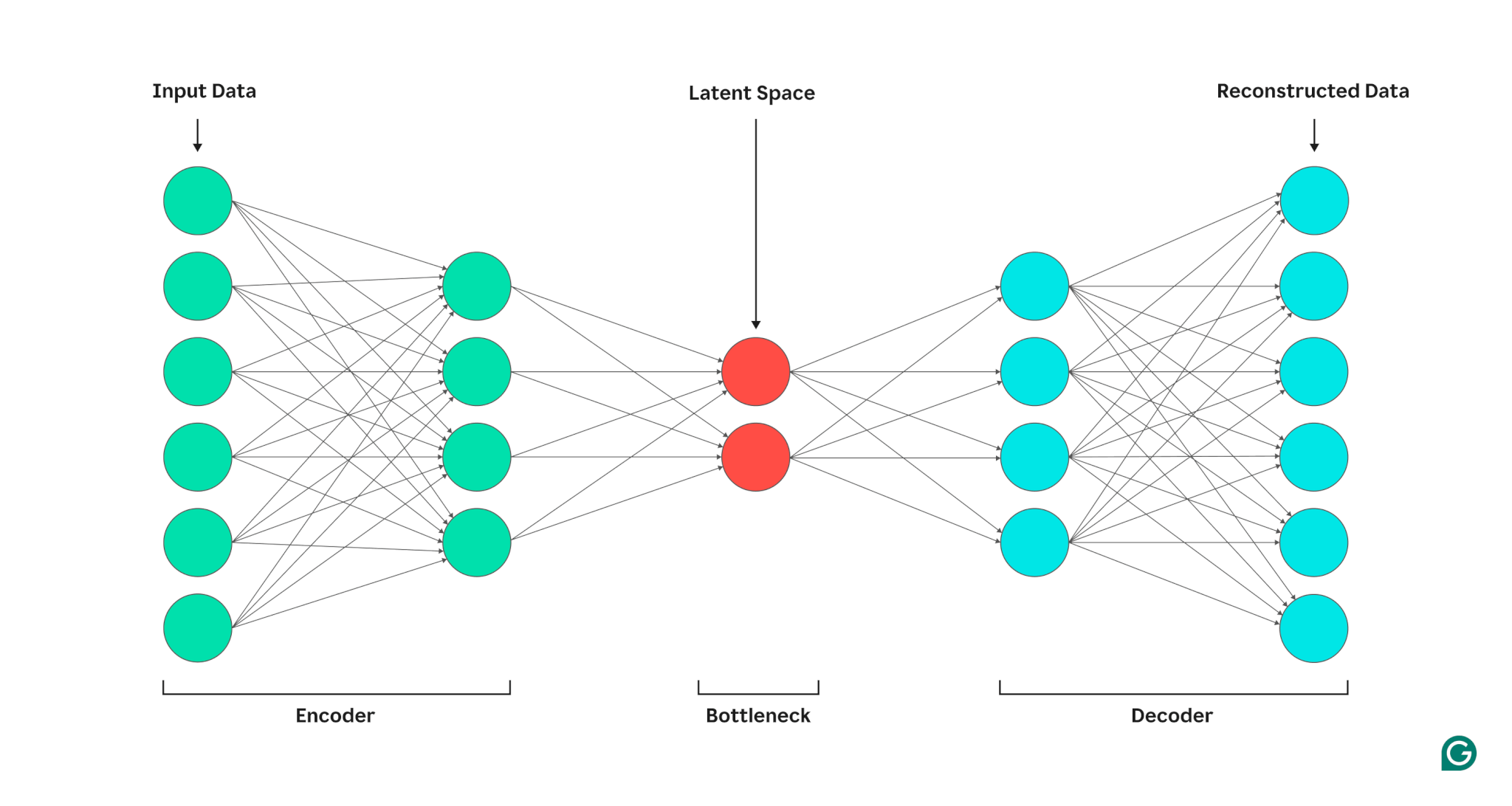
When you train a model to predict part of its input from another part (like a missing word in self-supervised models), an encoder compresses and distills the complex data into lower-dimensional, information-rich forms. The decoder then takes this rich representation to produce a structure output.
Researchers started to notice that the hidden layers weren’t just a step in solving the task but were building powerful intermediate representations embedded in the hidden layers — i.e., compressed versions of the input that strip away noise and highlight what matters. As shown below, they can map complex relationships in meaning between words and sentences.

They called them embeddings and began to harness their power. The embeddings started to serve as a general-purpose summary of everything important the model has learned about the input, which in turn could be reused for many different tasks like classification, translation, or sentiment analysis.
3. Putting It Together
At this point, machine learning has cracked two powerful ideas:
Self-supervised learning can train models without labeled data by hiding part of the input and making the model guess it
Embeddings hold useful internal representations that capture the essential and complex patterns and relationships inside the data
If you combine these two ideas, you could build models that don’t just classify or fill in missing words. You could actually generate language by predicting the next word over and over again.
This led to a shift from models built for single tasks to general-purpose language models that could adapt to many tasks with little or no extra training.
We’ll cover this in Part 2!
Go to Part 2 or the main page.
4. Appendix
4.1 Glossary
Activation function: A mathematical function applied to a neuron's output to introduce non-linearity, allowing the model to learn complex patterns (e.g., sigmoid function).
Backpropagation: The process of passing gradients backward through a neural network to update weights based on the chain rule, enabling training with gradient descent.
Batched gradient descent: A form of gradient descent where the gradient is computed over the entire dataset at once — accurate but slow for large datasets.
Bias term: A special input with a constant value (typically 1) that allows the model to learn an intercept in linear regression.
Cross-entropy loss: A loss function used in classification tasks (also called log loss) that measures the difference between predicted probabilities and actual labels.
Decoder: The part of a neural network that takes the encoded (latent) representation and transforms it back into a structured output — such as reconstructed input, translated text, or predicted next tokens.
Dot product: The weighted sum of inputs multiplied by their corresponding weights in a neuron — the core calculation of a linear model.
Embeddings: Compact, learned representations of inputs that capture meaningful features and can be reused across tasks.
Encoder: The part of a neural network that processes input data and transforms it into a compact, information-rich representation (called the latent space).
Epoch: One full pass through the entire dataset during training; often multiple epochs are needed for effective learning.
Features: The input variables given to a model to help predict an output (e.g., square footage, number of bedrooms).
Gradient: The vector of partial derivatives of the loss function with respect to model parameters, used to update parameters in gradient descent.
Gradient descent: An optimization algorithm that adjusts model parameters in the direction of the negative gradient to minimize the loss function.
Gradient functions: The partial derivatives of the loss function with respect to each parameter — used to calculate the gradients for updates.
Hidden Layer: The intermediate layers of a neural network between the input and output, where the model transforms and processes data.
Label: The correct output provided by a human (or source) in supervised learning, used to guide the model’s learning process.
Learning rate: A hyperparameter that controls the size of each update step during gradient descent to ensure stable convergence.
Linear regression: The simplest form of supervised learning where a straight line is fitted to predict outputs from inputs.
Log loss: Another name for cross-entropy loss, used in classification to penalize incorrect predictions based on probability.
Loss: A measure of how far off the model’s predictions are from the correct output, guiding the optimization process.
Loss function: A mathematical function that computes the error between predictions and actual values (e.g., Mean Squared Error).
Mean squared error: A common loss function for regression that squares the prediction errors and averages them across data points.
Model: A system that maps input features to outputs using learned parameters, aiming to minimize the loss.
Multi-layer perceptron (MLP): A neural network architecture with an input layer, hidden layers, and an output layer, allowing complex function approximation.
Neural network: A model made of interconnected layers of neurons that can learn complex mappings from inputs to outputs.
Non-linearity: The property added by activation functions that allows a neural network to model complex patterns beyond straight lines.
Overfitting: A modeling error where the model learns noise or quirks in training data instead of general patterns, hurting performance on new data.
Parameters: The weights (and biases) in a model that are adjusted during training to improve performance.
Perceptron: The basic unit of a neural network — a linear prediction followed by an activation function.
Samples: The individual data points used to train a model, each consisting of input features and (usually) a label.
Sigmoid function: A common activation function that maps inputs to a value between 0 and 1, used especially in binary classification.
Supervision: The concept of providing a model with labeled data (correct answers) during training in supervised learning.
Training cycle: The complete process of training a model, often involving multiple epochs over the dataset.
Training step: A single iteration of the training loop: making predictions, calculating loss, computing gradients, and updating parameters.
Unsupervised learning: A type of learning where the model finds patterns in data without explicit labels or supervision.
Weight: The adjustable parameter in a model that scales input features in prediction calculations.